Sean Dunn
Presented on 1/27/1999
CS563

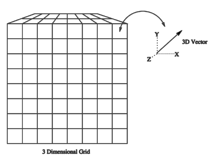
In this presentation we consider a field to be a 4D grid (in the x,y,z, and time dimensions) with uniform sampling distances along any dimension. At each grid point, there is a normalized vector which determines the direction of force local to that point.

Requirements of a Turbulent Wind Field [2]

Large and Small Flow Eddies

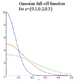
Energy fed into a turbulent system goes primarily to the larger eddies. Smaller Eddies are shed from these, and the process continues until the eddies become small enough for dissipation to occur. This phenomenon is called an energy cascade, and can be represented by a spectral function which shows the amplitude of spatial frequencies. An example of this is based on a Gaussian fall-off function:

where w is the frequency and c is a constant that a user can specify to customize the behavior of the function.

Periodicity in Space and Time

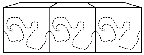
To create a grid of sufficient resolution, and also respect the limitations of state memory on a computer, making a grid that is periodic in space and time is a much better idea than creating one large world-encompassing one. This actually does not produce many noticeable aliasing effects. It can be thought of as a 4D tiled texture, using force vectors instead of colors.

Synthesizing Turbulent Wind Fields

Fourier Space

Fourier theory dictates that a discrete sampling of values over some dimension can be de-constructed into a series of sinusoidal waves (through what is known as the Fourier transform) that, when added, recreate the original wave sample. Numbers in Fourier space are complex, where the real component is the amplitude of the frequency, and the complex component is the phase.

An accessible analogy would be that of a graphic equalizer on a high end stereo. The graphic equalizer continuously samples the audio channel, and gives a readout of the sonic frequencies and Decibel levels each one of those frequencies is generating. If there existed a graphic equalizer that sampled the thousands of different frequencies within the human range of perception, and then summed them up, the result would be the original audio signal - effectively the inverse Fourier transform of the frequencies and amplitudes.

Graphic Equalizer/Fourier Transform Analogy

Fourier Synthesis

If we begin in Fourier space, with a spectral function of frequencies and amplitudes, we can apply the inverse Fourier transform to this function and create a synthetic waveform in dimensional space. This synthetic waveform can be considered a one-dimensional turbulence.

Applying this in three dimensions will generate a turbulence field in three dimensions. If we multiply the spectral function by a random noise function in Fourier space, we can then create multiple versions of this turbulence, using successive versions for sequential time frames.

Algorithm for Creating Turbulent Windfields [3]

Assume:

F is the R4 frequency domain array that the inverse DFT will operate upon.
G is the R4 space-time domain array that the inverse DFT will return.
x,y,z,t are integers used to index the above arrays
Nx, Ny, Nz, Nt are the dimensional sizes of the arrays
d,i,j,k,l are floating point numbers
r is a R3 floating point real vectors
u,v are R3 floating point complex vectors
B is a user specified turbulence parameter

for  t = 0 .. Nt {
     for z = 0 .. Nz {
          for y = 0 .. Ny {
               for x = 0 .. Nx {
	            i = x/Nx ; j = y/Ny ; k = z/Nz ; l = t/Nt   /* put into normalized form */
		    if (i > Nx/2)  i = i - 1     /* keep the values for the normalized values */
		    if (j > Ny/2)  j = j - 1     /* in [0 .. 0.5, -0.5 .. 0] instead of [0, .., 1] */
		    if (k > Nz/2)  k = k - 1                              
		    d = sqrt(i2 + j2 + k2) 	    /* compute distance from origin in normalized   space */
		    rx = uniform_random(0, 2*PI)       /* assign a statistically random number */
		    ry = uniform_random(0, 2*PI)       /* between 0 and 2*PI */
		    rz = uniform_random(0, 2*PI)

		    /* assign the Gaussian spatial frequency function S(w,c) (with w 
		    replaced with d, and c replaced with B) from above using the 
		    spatial distance and the user-specified parameter as arguments, as a 
		    complex number (a + bi), into a vector v (note: i is the complex number 
		    constant (i = sqrt(-1)), while i is the x-dimensional float iterator) */
		    vx = S(d, B) cos(rx) + S(d, B) sin(rx) i
		    vy = S(d, B) cos(ry) + S(d, B) sin(ry) i
		    vz = S(d, B) cos(rz) + S(d, B) sin(rz) i

		    /* project this vector onto a plane normal with <i,j,k> */
		    ux =  (1 - i2/d2)vx     -   (ij/d2)vy     -    (ik/d2)vz
		    uy =     - (ij/d2)vx + (1 - j2/d2)vy    -    (jk/d2)vz
		    uz =    - (ki/d2)vx    -   (kj/d2)vy + (1 - k2/d2)vz

		    /* Set the F array value at the current indice to u, and set the value at the diagonally correlated 
		    indice in this array to the complex conjugate of u (denoted by u*)                                          */ 
		    F(x,y,z,t) = u
		    F((Nx-x)%Nx, (Ny-y)%Ny, (Nz-z)%Nz, (Nt-t)%Nt) = u*
               }
          }
     }
}

/* set the imaginary values at the 0 and N/2 indices to 0.0 for correct symmetry
in the calculation o */
for  t = 0, Nt/2 {
     for z = 0, Nz/2 {
          for y = 0, Ny/2 {
               for x = 0, Nx/2 {
	            Fimaginary(x,y,z,t) = 0.0
               }
          }
     }
}

/* Calculate the inverse DFT in the 4 dimensions of F, for one vector component at a time,  
then normalize the resulting vector lengths in the range of [-1..+1] */
Gx = InverseDFT4D(Fx)
Gy = InverseDFT4D(Fy)
Gz = InverseDFT4D(Fz)

Normalize(G)

Synthesized Turbulent Vector Field (11.3Mb AVI)

Hypercube Interpolation

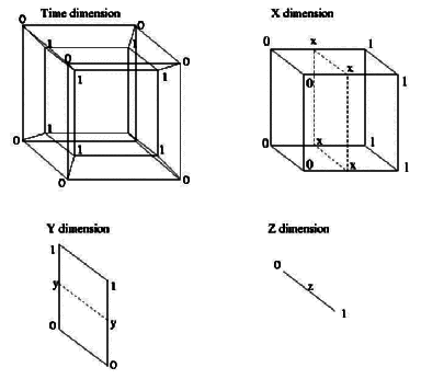
If we evaluate the turbulence force at a point in space that does not exactly correspond to the placement of vector grid points in space, we can perform a quadrilinear interpolation. The geometric equivalent of a 4 dimensional shape is the Hypercube. For each dimension (including time), we reduce our original 16 vectors by squashing into the next dimension down (and interpolating linearly in that dimension), until we have a single vector, which is the linear combination of the original 16. We can also convert the vectors from cartesian space to spherical space before doing this to make transition between vector angles more constant.

Advection of Particles in a Turbulent Wind Field (7.9Mb)
Diffusion of Smoke Particles in a Turbulent Wind Field (954Kb AVI)

Implicit Surfaces

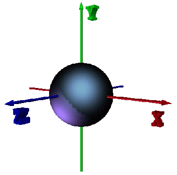
Implicit surfaces are isosurfaces, surfaces defined through some scalar field in 3D (at which all points on the surface yield an equal value according to an evaluation function). An example would be the simple equation:

for which a sphere can be realized as the shell surrounding the origin where D(x,y,z)=1.

Blobby Models (Blinn's Electric Field Model)

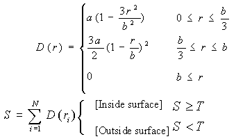
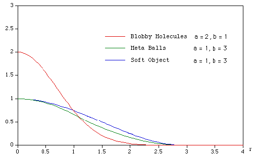
The use of implicit surfaces in computer graphics was first accomplished by Blinn [1], as a way of simulating the smooth cover of electron density fields (van der Waals surfaces) which he called "blobby models".

r is the distance from the center point of an atom, a is the height of the function at r=0, and b is related to the standard deviation of the curve, which is a Gaussian. At any surface point, the isosurface "potential" is equal to the sum of all the neighboring atoms' contributions using this function:

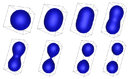
where N is the total number of blobs (atoms) and T is a threshold constant that determines the value of the isosurface. As T increases, the surface gets more compact and smoother between adjacent "blobs".

Metaballs

A computationally cheaper alternative to using Blinn's basis function is the piecewise polynomial developed at Osaka University in Japan. Implicit surfaces created with this method are called "metaballs" (rumored to be a forced misspelling of "meatballs"). This function is:

where a is the value of D(r) at r=0, and b is the root of the equation. For all r>b, the function returns 0. The behavior of this function is very similar to that of the "soft objects" of Wyville, McPheeters, and Wyville, that Professor Ward [5] had presented in his January 20th lecture.

Graphs of Three Basic Functions

The following is a graph showing the relationship of the metaball, soft object, and blobby model basis functions:

Example of Metaballs in Action [2]

An even smoother transition between blobs could be achieved by increasing b, the "radius of involvement" with neighboring blobs.

Volume Raycasting

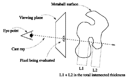
To render an implicit surface volume one can employ a simple ray casting algorithm that will sample discrete points along an imaginary line in 3D space. Although much slower than other visualization techniques, such as marching cubes, it is very useful in rendering models of natural phenomena, such as fire, where the intersected length of the ray with the blob is proportional to the amount of energy (light) being emitted along that ray to the camera point.

Backwarping Implicit Surfaces Through Turbulent Wind Fields [3]

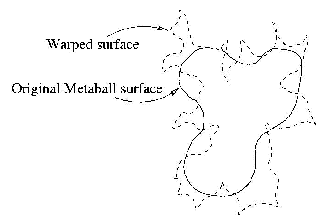
Backwarping can be considered the same as "pushing" our blobby model through the wind field. A more abstract and functional description is that we are "pushing" our evaluator points through the windfield. When the cast ray from the renderer evaluates a point in space, that evaluation point is warped itself, which gives the end illusion of the blobby model being warped.

Visual Examples

Realistic Candle Flame (690Kb AVI)


In this simple metaball particle system, a coloring function (based on thickness of the surface and height of the flame) was applied to the rendered object. A small amount of backwarping turbulates the metaball surface, while the position of the metaball particles are also under influence from the wind field as they rise to give the illusion of flicker.

Smooth Fire (698Kb AVI)


Here, a hard-coded coloring function (based only on thickness) was employed to color the flames emanating from this blob particle system. Like the above example, the blob particle positions are also under influence from the wind field.

Turbulent Fire (1.1Mb AVI)


Here, the previous example was copied into four different positions in the scene, and the turbulence was raised, as well as the speed of the rising particles.

A Cloud(34Kb GIF)


This is a major hack to simulate a cloud by diffusing metaball particles generated on a disc in space, and then applying a simple blue-gray-white coloring function based on thickness. Major turbulence was introduced to pull out the whisps of the cloud.

References

[1] Blinn, J., "A Generalization of Algebraic Surface Drawing," ACM Transactions on Graphics, Vol. 1, No. 3, pp. 235-256, July, 1982.

[2] Bourke, Paul, "Implicit Surfaces," June 1997,
http://www.mhri.edu.au/~pdb/modelling/implicitsurf/.

[3] Stam, Jos and Eugene Fiume, "Turbulent Wind Fields for Gaseous Phenomena", Proceedings of SIGGRAPH `93. In Computer Graphics Proceedings, ACM SIGGRAPH, 1993, 369-376.

[4] Stam, Jos, "A General Animation Framework for Gaseous Phenomena," ERCIM Research Report R047, January 1997.

[5] Ward, Matt, "An Overview of Metaballs/Blobby Objects,"
http://www.cs.wpi.edu/~matt/courses/cs563/talks/metaballs.html.