![[Return to the CS 563 Homepage]](http://www.cs.wpi.edu/images/back.gif)
Presented by Sean Dunn on 3/31/1999
CS563
Today's graphics applications require CG imagery to combine seamlessly with photographed images. An accurate model of the photographics process could greatly benefit this.A photographed and digitized picture is simply an array of brightness values. These values rarely correctly map to true measurements of the relative radiance in the scene. There is actually a compositing of several unknown, nonlinear mappings that determine the brightness of a pixel in a scene.
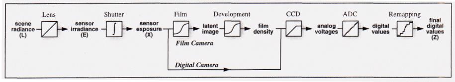
The exposure of the film is a nonlinear product of E (the irradience constant) and deltaT(the exposure time). Thus, the relationship between the scene radiance L and the final pixel value Z is also nonlinear. Digital imaging devices introduce their own nonlinear mapping so that the produced image mimics actual film stock more closely, corrects for the non- linearity of the CCD device, and sometimes to convert from the 12bit hardware color channel output to the 8bit values used in many types of image media.What this paper accomplishesThe algorithms presented in this paper take in a set of images acquired over a range of exposure times, and uses this information to approximate the original non-linear characteristic function of the film - and also to generate a radiance map of the scene, which will show the entire dynamic radiance range caught by the original photograph.
Image Processing
Most image processing operations (blurring, edge detection) assume pixel values to be proportional to the scene radiance. Because of the nonlinearity of scene radiance (especially saturation points), these operations can produce incorrect results.
Image Compositing
Many applications of computer graphics involve combining (compositing) different images acquired using wholly different methods. Ex: a background shot with a still camera, with an overlay image shot with motion picture film stock, and CG effects elements overlayed onto this. A correct model of the radiance functions of each of these elements would allow them to be more seamlessly integrated.
This is algorithm exploits a principle of photochemical and electronic imaging systems known as reciprocity. The response of film to variatons in exposure is characterized by its Hurter-Driffield curve, or, its "characteristic" curve:
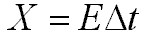
X is the total exposure, while E and deltaT are the radiance and exposure times, respectively. Reciprocity states that if we halve the value of E and double the value of deltaT, we will get the same value for X.
After the developing and scanning of an image, we have a digital value Z, which is a nonlinear aggregate function of X:
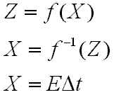
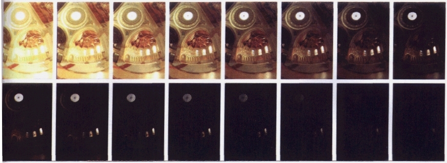
The input to this algorithm is a set of digitized photographs taken from the same orientation in space, with different known exposure times deltaTj. We assume that the lighting does not change over time - or - Ei for each pixel i is constant. Pixel values are denoted by Zij where i is the spatial index, and j is the index into the exposure time of the image.
The film reciprocity equation can be written as:
We can take the natural log of both sides to get:
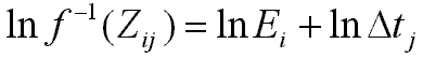
ln f-1 can be simplified as g:

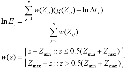
Letting Zmax be the brightest pixel values, and Zmin be the least brightest value, our pixel range becomes (Zmax - Zmin + 1). N is the number of pixel locations, and P is the number of photographs. The problem now becomes on of finding the (Zmax - Zmin + 1) values of g(z) and the N values of Ei that minimize the following quadratic objective function:
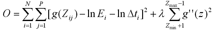
The first term ensures that, in a least squares sense, that g(z) is satisfied - the second term is a smoothing function that ensures that g(z) is smooth.
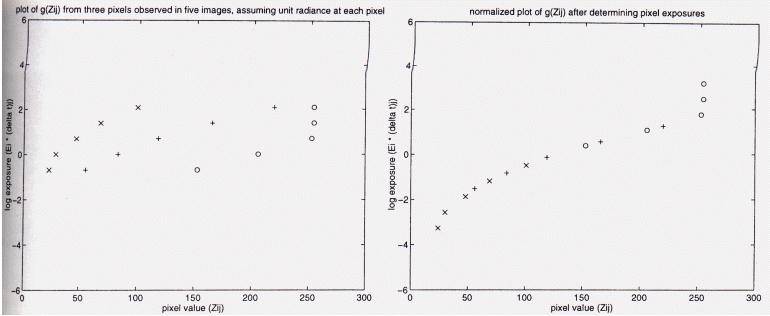
Basically, we slide our samples vertically until they meet smoothly. Voila - a characteristic function curve.
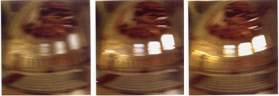
Gaussian motion blur (left), Real film motion blur (center), Synthetic motion blur using these techniques (right)
[1] Debevec, P., Jitendra Malik, "Recovering High Dynamic Range Radiance Maps From Photographs," SIGGRAPH Proceedings 1997, pp. 130-135.