XmdvTool User's Manual
Menu: File
Command - Open:
Function:
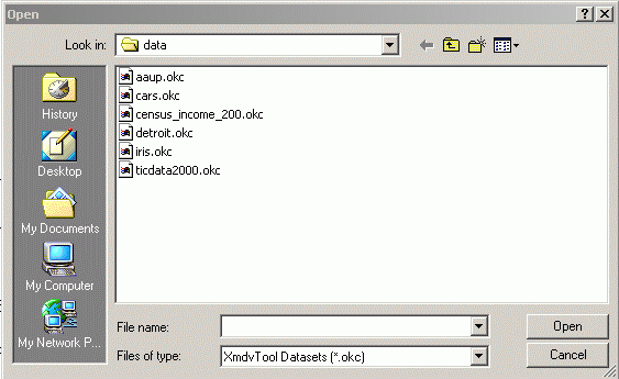
Raise a standard file open dialog. You can open a new data set through this dialog.
Operation:
The data set must have a name of *.okc and must be in okc format. Open the *.okc file through the standard file open dialog.
Tips:
okc format:
The expected input format of a data set in XmdvTool. Here is an example data set "example.okc":
4 3
sepal_length
sepal_width
petal_length
petal_width
5.200000 5.700000 5
4.100000 4.400000 5
1.400000 1.500000 5
0.100000 0.400000 5
5.700000 4.400000 1.500000 0.400000
5.200000 4.100000 1.500000 0.100000
5.500000 4.200000 1.400000 0.200000
Explanation of this data set is:
4 3
* This data set contains 4 dimensions, three data items
sepal_length
* The name of the first dimension is "sepal_length".
Dimension names should not contains blank space.
sepal_width
* The name of the second dimension.
petal_length
* The name of the third dimension.
petal_width
* The name of the fourth dimension.
5.200000 5.700000 5
* In this data set, all the values of the first
dimension are in the range [5.200000 5.700000].
* When this dimension is discreet, it is divided
into 5-1 = 4 uniform ranges.
4.100000 4.400000 5
* Range of the second dimension. When this
dimension
* is discrete, it is divided into 5-1 = 4 uniform
ranges.
1.400000 1.500000 5
* Range of the third dimension. When this dimension
* is discrete, it is divided into 5-1 = 4
uniform ranges.
0.100000 0.400000 5
* Range of the fourth dimension. When this dimension
* is discrete, it is divided into 5-1 = 4
uniform ranges.
5.700000 4.400000 1.500000 0.400000
* The first data item's value at the first dimension is 5.700000,
at the second dimension
* is 4.400000, at the third dimension is
1.500000, fourth 0.400000.
5.200000 4.100000 1.500000 0.100000
* The value of the second data item.
5.500000 4.200000 1.400000 0.200000
* The value of the third data item.
Automatic clustering function:
In previous versions of XmdvTool, you have to generate a data hierarchy yourself if you want to view the data set in a multi-resolution manner. Now you no longer need to do that. The system will automatically generate the cluster file in binary format for you if you have not provided one. If you want to generate your own cluster file, you will have to use a translation tool referred on the xmdv web page, for converting from .okc to .cg/.cf:
http://davis.wpi.edu/~xmdv/downloadtools.html
For more Datasets:
http://davis.wpi.edu/~xmdv/datasets.html
Tools for converting to .okc format:
http://davis.wpi.edu/~xmdv/downloadtools.html
Back to top
Command - Close:
Function:
Close the current data set.
Back to top
Command - Save Image:
Function:
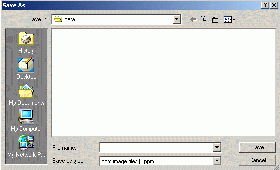
Save the current display in the main window as an image in the ppm format.
Operation:
Input the image file name into the standard Save As dialog, then click the Save button.
Tips:
You can save the brushed data into a new data set for recording an interesting pattern or for further exploration of a subset of a data data.
Back to top
Command - Save Brushed Data:
Function:
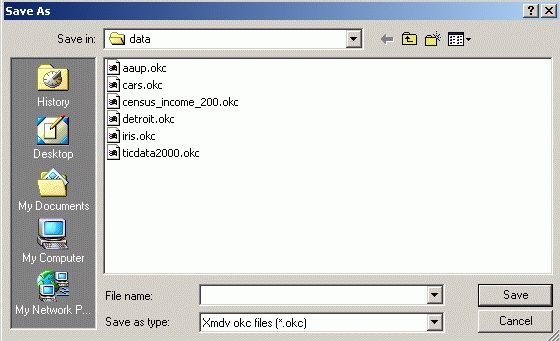
Save the brushed data as a new data set in the okc format.
Operation:
Input the name of the new data set into the standard Save As dialog. then click the Save button.
Tips:
You can use this command to generate new data sets. You can open them using Command Open.
Back to top
Command - Quit:
Function:
Quit XmdvTool.
Tips:
You can also quit XmdvTool by clicking the X icon on the right up corner of the main window.
Menu: Tools
- Manual Dimension On/Off/Reorder
- Automated Dimension Reordering
- Dimension Reduction
- Data Summary & Statistics
- Glyph Customization
- Time Series Animation
Command - Manual Dimension On/Off/Reorder:
Function:
Raise the Dimension On/Off/Reorder Dialog to enable you to manipulate dimensions, such as to turn on, turn off some of the dimensions, or reorder the dimensions.

Operation:
-
Check the "On" field after a dimension name to turn the dimension on.
-
Uncheck the "On" field after a dimension name to turn the dimension off.
-
Click the "<-" button after a dimension name to increase the dimension's order. If it is already the first dimesion, it will become the last one.
-
Click the "->" button after a dimension name to decrease the dimension's order. If it is already the last one, it will become the first one.
Tips:
-
When a dimension is turned off, you will not see it from the displays.
-
You can change the order of the dimensions to change the adjacent relationships of the dimensions.
-
When there are too many fields to fit in this dialog, use the horizontal and vertical scrolling bars to see rest of the fields.
Back to top
Command - Automated Dimension Reordering
Function:
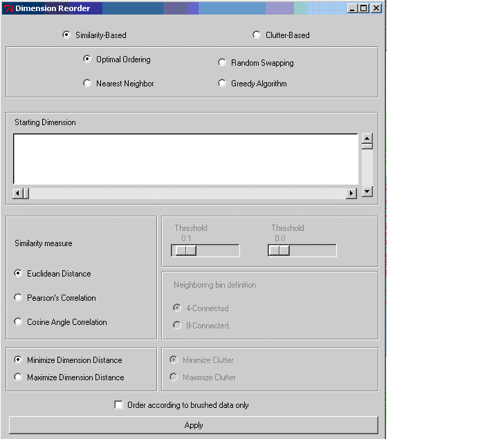
Various parameters and thresholds can be set by the user to better control the reordering process. Dimension reordering dialog box allows you to set the parameters for reordering dimensions according to two criteria: dimension similarities or visual clutter.
Operations:
In this Dimension Reorder dialog box, the user should first specify whether to reorder the dimensions using a similarity measure or a clutter measure.
1) Similarity-Based Dimension Reordering Parameters
Each similarity measure reveals dimension relationships in a different way.
- Check any one of the radio button “Euclidean Distance”, "Pearson's Correlation" or "Cosine Angle Correlation" to select it as a similarity measure.
- Check the radio button “Minimize/Maximize Dimension Distance” to reorder dimensions to minimize or maximize total distances between neighboring dimensions.
2. Clutter-Based Dimension Reordering Parameters
- “Threshold scale” allows the user to specify the thresholds in the four visualization techniques (Parallel Coordinates, Scatterplot Matrices, Star Glyphs and Dimension Stacking).
- “4-Connected or 8-Connected” radio buttons allow the user to indicate which neighbor definition to use in dimensional stacking visualization.
- “Minimize/Maximize Clutter” radio buttons allows you to reorder dimensions to minimize or maximize total visual clutter in the display.
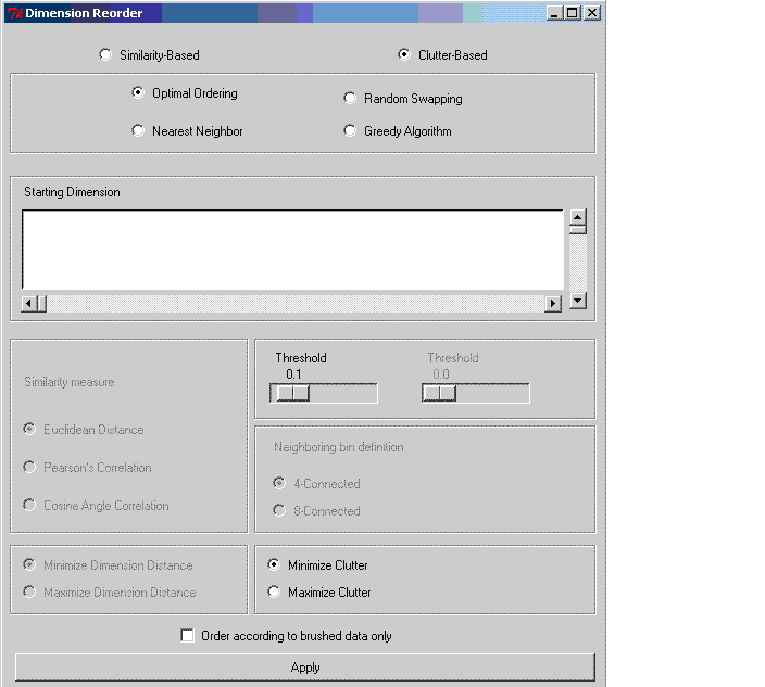
3. General Reordering Parameters
Reordering Algorithms allow the user to use four different algorithms to search for a desired dimension order.
- Check the radio button “optimal algorithm” to reorder dimensions by doing an exhaustive search.
- Check on the “random swapping” to reorder dimensions using random swap.
- Check on the radio button “Nearest neighbor” to reorder dimensions using the nearest neighbors. A list of available dimensions is provided to enable the user to pick the starting dimension in nearest neighbor algorithm.
- Check on the radio button “greedy algorithm” to reorder using a greedy algorithm.
- “Brushed Data only” check button allows you to reorder dimensions according to a subset of the data items specified by using the manual Brushing functionality of the XmdvTool.
Tips:
The definitions of thresholds in the Clutter Based Dimension Reordering are:
- Parallel Coordinates: Normalized Euclidean distance between two data points. If the distance between two points is less than the threshold, they are considered clustered, otherwise not.
- Scatterplot Matrices: - Threshold 1: The difference between the Pearson Correlation Coefficient of two plots. If the difference is less than the threshold, the two plots are considered similar, otherwise not. - Threshold 2: The ratio of a dimension's cardinality and the pixel number of a plot's short side. If the ratio is greater than the threshold for a dimension, it is considered high-cardinality dimension, otherwise low-cardinality.
- Star Glyphs: - Threshold 1: The length difference between two neighboring rays. If the difference is less than the threshold, the two rays are considered positioned properly, otherwise not. - Threshold 2: The length difference between two symmetric rays. If the difference is less than the threshold, the two rays are considered positioned properly, otherwise not.
- Dimensional Stacking: The number of minimum aggregated bins. If a cluster has more bins than the threshold, the points of the cluster are considered “clustered”, otherwise these points are considered isolated outliers.
Command - Dimension Reduction:
Function:
Raise the Dimension Reduction Dialog so that you can reduce the dimensionality of the display using the Visual Hierarchical Dimension Reduction (VHDR). Please refer to the help page of Dimension Reduction.
Back to top
Command - Data Summary & Statistics:
Function:
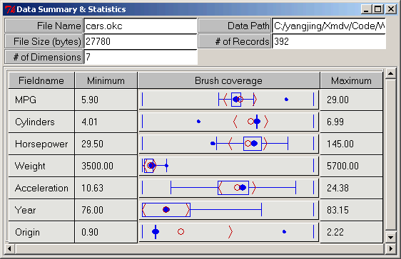
Raise the Data Summary & Statistics Dialog to provide you the data summary and statistics information of the current data set.
Back to top
Command - Glyph Customization:
Function:
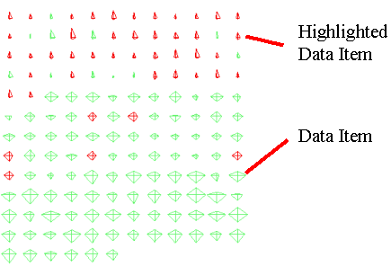
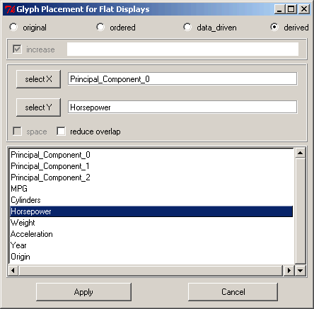
Raise the Glyph Placement for Flat Display Dialog. You can change the glyph placement mode for flat displays.
Operation:
There are four different glyph placement modes in XmdvTool:
-
Original - Glyphs are placed from left to right, then up to down, according to their order in the *.okc file.
-
Ordered - Glyphs are placed from left to right, then up to down, according to their values in one dimension (base dimension).
-
Data_driven - Glyphs are plotted in the display according to their values in two dimensions (X dimension and Y dimension).
-
Derived - Glyphs are plotted in the display according to two of their principal components or dimensions values.
To select the Original mode, check the "original" radio button on the top of the dialog, then click the "Apply" button at the bottom.
To select the Ordered mode:
-
Check the "ordered" radio button on the top of the dialog.
-
Click one of the dimensions listed in the list box as the base dimension.
-
Check the "increase" check button for an increasing order. Uncheck it for an decreasing order.
-
If you check the "space" check button, the distance between two adjacent glyphs will be proportional to the difference of their value in the base dimension.
-
Click the "Apply" button at the bottom.
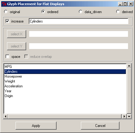
.
To select the Data_driven mode:
-
Check the "data_driven" radio button on the top of the dialog.
-
Click one of the dimensions listed in the list box as the X dimension. Click the "Select X" button to make it to appear in the entry after the button.
-
Click one of the dimensions listed in the list box as the Y dimension. Click the "Select Y" button to make it to appear in the entry after the button.
-
If you check the "reduce overlap" check button, the overlapped glyphs will be separated a little bit..
-
Click the "Apply" button at the bottom.
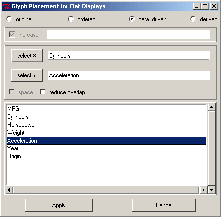
.
To select the Derived mode:
-
Check the "derived" radio button on the top of the dialog.
-
Click one of the principal components or dimensions listed in the list box as the X dimension. Click the "Select X" button to make it to appear in the entry after the button. Principal_Component_0, Principal_Component_1, Principal_Component_2, are the first, second, and third principal components of the data set.
-
Click one of the principal components or dimensions listed in the list box as the Y dimension. Click the "Select Y" button to make it to appear in the entry after the button.
-
If you check the "reduce overlap" check button, the overlapped glyphs will be separated a little bit.
-
Click the "Apply" button at the bottom.
Tips:
You can see the change of glyph placement immediately after you click the "Apply" button.
Back to top
Command - Time Series Animation
Function:
The Time Series Animation dialog box allows users to set the parameters and control time series animation.
Operation:
1) Selecting Time Dimension:
Time series animation displays the records according the order of one dimension. Time dimension widgets allow users select a dimension. Select a dimension in the combo box, and then click the “Select Time Dimension” button, that dimension will become time dimension.

Figure 1: Time Dimension Dialog
2) Setting Time Window Width:
Time window width controls window size, and only records that fall in this window will be shown. Users can move the slide bar to select time window width.
3) Setting Current Time:
While animation is playing, current time widget shows the center of displayed records.
4) Manual Option:
When manual is checked, users can move the Current Time manually and watch the selected records.
5) Selecting Style:
Select a style for animation color. Four styles are available: “Green->Yellow”, “Fade out”, “Red-Blue”, “Red->Blue, Fade out”.
6) Animation:
Click this button, the animation will be played.
Tips:
- The range of time window width is from 0.10 to span of the selected of dimension, which is the difference between the maximum value and the minimum value of the selected of dimension.
Menu: View
- Display Mode
- Auxiliary Display
- Toolbar
- Zoom Controls
- Glyph Key
- Dimensional Stacking Key
- Color Requester
- Font Name
- Font Size
- Distortion
Cascade - Display Mode:
Function:
Change the current display mode of the main window.
Operation:
Click the display mode you want in the cascade. Details of each display mode can be found in the "Term Explanation" in the Help Dialog.
Tips:
You can view two different display modes at the same time by using the Auxiliary Display from the "View" menu.
Back to top
Command - Auxiliary Display:
Function:
Raise the Auxiliary Display Dialog so that you can view two different display modes at the same time (one in the main window, the other in the Auxiliary Display Dialog).
Operation:
Click the "Select a Display" button in the top of the Auxiliary Display Dialog to raise a cascade. Click a display mode you want from the cascade.
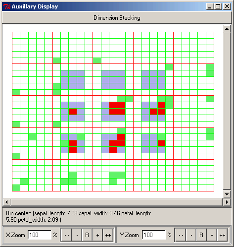
For example, select the "dimensional stacking" mode, and the display will be:
Tips:
Tips: There is zooming function in this dialog to control the auxiliary display. Any cursor or hotkey operation that works on the display in the main window will also work in this display.
Back to top
Check Button - Toolbar:
Function:
Raise/hide the toolbar.
Operation:
Check it to raise the toolbar. Uncheck it to hide the toolbar.
![]()
Tips:
1. There are zoom entries and some useful quick buttons on the toolbar, such as “open”, “Color Requester”, “Struct-based brush”. Clicking them is the same as clicking the corresponding command from the menu.
2.When you place the cursor on a quick button, the name of the corresponding command of that quick button will be displayed in the message bar (it is in the bottom of the main window) .
Back to top
Check Button - Zoom Controls:
Function:
Raise/hide the toolbar. When the toolbar is raised, you may zoom the display in the main window using the zoom entries in the toolbar.
Operation:
![]()
To zoom in the display in X direction, either click the + or ++ button after the X Zoom label. To zoom out the display in X direction, either click the - or -- button after the X Zoom label. To reset the display in X direction, click the R button after the X Zoom label. You can also directly input the zoom factor into the entry after the X Zoom label followed by pressing “enter” key.
When the display is X zoomed in, you can move the focus of the display by dragging and dropping the horizontal scrolling bar around the display..
Zooming in Y direction is similar to zooming in X direction. X Zoom and Y zoom are independent form each other.
Tips:
1. ++ leads a larger increase than + does. - - leads a larger decrease than -.
2. Many dialogs contain displays. Usually they contain similar zoom entries as the zoom entries in the toolbar. You can zoom those displays in the same way using their zoom entries.
Back to top
Command - Glyph Key:
Function:
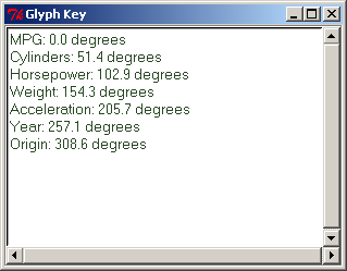
Raise the Glyph Key Dialog to provide you the dimension information for the Glyphs display.
Example:
When the Glyph shape is Star Glyph, the Glyph Key Dialog will give information about each dimension (dimension name and angle degree in the star glyphs).
Back to top
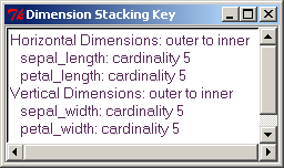
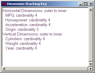
Command - Dimensional Stacking Key:
Function:
Raise the Dimensional Stacking Key Dialog to provide you the dimension information for the dimensional stacking display.
Back to top
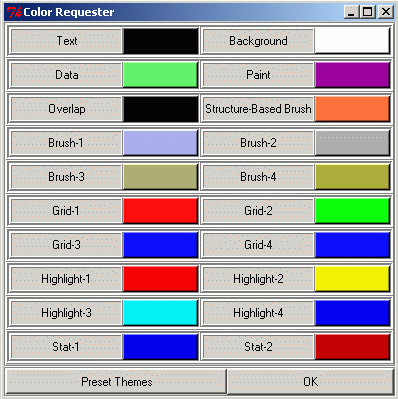
Command - Color Requester:
Function:
Raise the Color Requester Dialog. You can change colors of text, data, highlight, grids, …. through this dialog..
Operation:
You can either click the colorful buttons to change a particular color, or use our pre-defined themes from the "Preset Themes" button in this dialog.
Example:
To change the text color, click the button on the right side of the label “TEXT”. A standard color selection dialog will be raised. Select the color you want from it, then click OK. You will see that the color of the text has been changed to the color you selected.
Tips:
1. Try the preset themes! You would like some of them! .
2. You need NOT close the Color Requester Dialog to see the effects.
3. You may refer to "Term Explanation" in the Help Dialog to find out the meaning of the different labels.
Back to top
Cascade - Font Name:
Function:
Change the menu font style.
Operation:
Click the style name you prefer from the cascade.
Back to top
Cascade - Font Size:
Function:
Change the menu font size.
Operation:
Click the font size you prefer from the cascade.
Back to top
Cascade - Distortion:
Function:
Enable/disable/reset distortion on the displays in the main window and the Auxiliary Display Dialog. With distortion, you can view details within context.
Operation:
-
Click "Start" from the cascade to enable distortion.
-
Click "Start" from the cascade to enable distortion.
-
Click "Reset" from the cascade to reset the displays back to the original states.
Tips:
When distortion is enabled, if the current display is
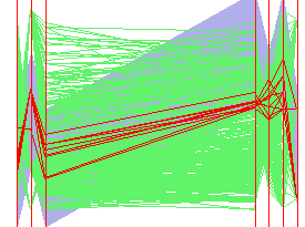
- Parallel Coordinates or Hierarchical Parallel Coordinates: click the left or right mouse button between two axes will increase the distance between them.
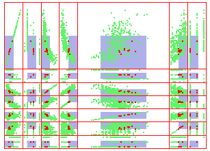
- Scatterplots or Hierarchical Scatterplots: Right mouse click in a plot will increase the area of the plot.
Examples:
1. Distorted Parallel Coordinates:
2. Distorted Scatterplots:
Back to top
Command - Auxiliary Display:
Function:
Raise the Auxiliary Display Dialog so that you can view two different display modes at the same time (one in the main window, the other in the Auxiliary Display Dialog).

Operation:
Click the "Select a Display" button in the top of the Auxiliary Display Dialog to raise a cascade. Click a display mode you want from the cascade.
For example, select the "dimensional stacking" mode, and the display will be:

Tips:
Tips: There is zooming function in this dialog to control the auxiliary display. Any cursor or hotkey operation that works on the display in the main window will also work in this display.
Back to top
Check Button - Toolbar:
Function:
Raise/hide the toolbar.
Operation:
Check it to raise the toolbar. Uncheck it to hide the toolbar.
![]()
Tips:
1. There are zoom entries and some useful quick buttons on the toolbar, such as “open”, “Color Requester”, “Struct-based brush”. Clicking them is the same as clicking the corresponding command from the menu.
2.When you place the cursor on a quick button, the name of the corresponding command of that quick button will be displayed in the message bar (it is in the bottom of the main window) .
Back to top
Check Button - Zoom Controls:
Function:
Raise/hide the toolbar. When the toolbar is raised, you may zoom the display in the main window using the zoom entries in the toolbar.
Operation:
![]()
To zoom in the display in X direction, either click the + or ++ button after the X Zoom label. To zoom out the display in X direction, either click the - or -- button after the X Zoom label. To reset the display in X direction, click the R button after the X Zoom label. You can also directly input the zoom factor into the entry after the X Zoom label followed by pressing “enter” key.
When the display is X zoomed in, you can move the focus of the display by dragging and dropping the horizontal scrolling bar around the display..
Zooming in Y direction is similar to zooming in X direction. X Zoom and Y zoom are independent form each other.
Tips:
1. ++ leads a larger increase than + does. - - leads a larger decrease than -.
2. Many dialogs contain displays. Usually they contain similar zoom entries as the zoom entries in the toolbar. You can zoom those displays in the same way using their zoom entries.
Back to top
Command - Glyph Key:
Function:
Raise the Glyph Key Dialog to provide you the dimension information for the Glyphs display.
Example:
When the Glyph shape is Star Glyph, the Glyph Key Dialog will give information about each dimension (dimension name and angle degree in the star glyphs).

Back to top
Command - Dimensional Stacking Key:
Function:
Raise the Dimensional Stacking Key Dialog to provide you the dimension information for the dimensional stacking display.

Back to top
Command - Color Requester:
Function:
Raise the Color Requester Dialog. You can change colors of text, data, highlight, grids, …. through this dialog..
Operation:
You can either click the colorful buttons to change a particular color, or use our pre-defined themes from the "Preset Themes" button in this dialog.
Example:
To change the text color, click the button on the right side of the label “TEXT”. A standard color selection dialog will be raised. Select the color you want from it, then click OK. You will see that the color of the text has been changed to the color you selected.
Tips:
1. Try the preset themes! You would like some of them! .
2. You need NOT close the Color Requester Dialog to see the effects.
3. You may refer to "Term Explanation" in the Help Dialog to find out the meaning of the different labels.
Back to top
Cascade - Font Name:
Function:
Change the menu font style.
Operation:
Click the style name you prefer from the cascade.
Back to top
Cascade - Font Size:
Function:
Change the menu font size.
Operation:
Click the font size you prefer from the cascade.
Back to top
Cascade - Distortion:
Function:
Enable/disable/reset distortion on the displays in the main window and the Auxiliary Display Dialog. With distortion, you can view details within context.
Operation:
-
Click "Start" from the cascade to enable distortion.
-
Click "Start" from the cascade to enable distortion.
-
Click "Reset" from the cascade to reset the displays back to the original states.
Tips:
When distortion is enabled, if the current display is
- Parallel Coordinates or Hierarchical Parallel Coordinates: click the left or right mouse button between two axes will increase the distance between them.
- Scatterplots or Hierarchical Scatterplots: Right mouse click in a plot will increase the area of the plot.
Examples:
1. Distorted Parallel Coordinates:

2. Distorted Scatterplots:

Menu: Brushes
All brush related operations are included in this menu, including flat brushes and hierarchical brushes.
- Brush Toolbox for Flat Displays
- Brush Data Value Dialog for Flat Displays
- Flat Parallel Coordinates Brush Toolbox
- Flat Glyphs Brush Toolbox
- Flat Dimensional Stacking Brush Toolbox
- Structure-Based Brush for Hier Displays
- Structure-Based Brush Semantics
Command - Brush Toolbox for Flat Displays:
Function:
Raise the Brush Toolbox Dialog. You can manipulate the brushes for the flat displays in this dialog.
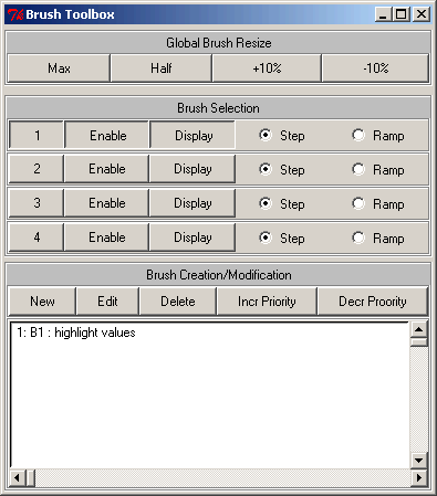
Global Brush Resize:
To: Adjust the size of the brush in all dimensions at once.
Do: Click on Max to have the brush cover the whole data set, Half to cover half of the range of the data (centered), +10 to increase the brush in all dimensions by 10 percent, and -10 do decrease the brush size in all dimensions by 10 percent.
Brush Selection:
To: Enable up to 4 brushes at once.
Do: Click on the Enable button for the brush you wish to enable.
To: Show the background for any brush.
Do: Click on the corresponding Display button.
To: Enable a brush to be modified in either the data display or one of the auxiliary brush dialog tools.
Do: Click on the numbered button of the brush you wish to change.
To: Enable switch between step and ramped brush boundaries.
Do: Click on either Step or Ramp for the brush you wish to modify.
Tips:
A ramped brush means that the brush has 2 sets of boundaries - one for points that are considered completely within the brush and one for points that are partially covered by the brush. The intensity of the brushed points decrease linearly between the inner boundary and the outer boundary. The outer boundaries may be modified in any data display by holding the Ctrl key down while moving the mouse. This has the affect of modifying the slope of the ramp.
Brush Creation/Modification:
To: Specify the function, structure, and priority of brushes.
Do: Clicking on New will open up the Brush Operation Toolbox to let you specify the operation and expression associated with a brush. The default for Brush 1 is highlight and enable display of values in an auxiliary display. This will create a new entry in the list box. To delete an existing brush, click on the brush in the list and Click Delete. To edit the operation or expression for an existing brush, click on the brush in the list and then click Edit. To change the priority of a brush, which determines what brush color will be displayed for a data point covered by multiple brushes, click on the brush you'd like to change the priority of and click either Incr Priority or Decr Priority.
Tips:
Just Enabling the dimension in the upper part of this dialog does not create the brush. You first have to create it in Brush Creation/Modification, and then you can Enable/Disable/Display it.
Brush Operation Toolbox

Brush operations are the actions that are to be performed on data selected by
the brush. XmdvTool supports four types of brush
operations: highlight, mask, values, and average. Each of these are
explained in detail below. In order to specify a brush operation the
Operation Toolbox must be used.
Highlight -- This operation causes all the points covered by the brush to be displayed in a different color. When this operation is active, the color will be available in the Color Requester .
Mask -- This operation causes all points covered by the brush to be hidden from the display. This is useful when the display is cluttered and it is necessary to remove some data to view other interesting data.
Values -- This operation causes the numeric value of all points covered by the brush to be displayed in a separate popup window. This window can be opened from the main interface by selecting Data Values.
Average -- This operations causes the average value of all points currently selected by the brush to be displayed in each of the display views. In addition, if the Values operation is also selected, the numeric average is added to the end of the values in the data values window.
Brush Expression
The brush expression is a logical expression between brushes. Points
are covered by the operation if they evaluate to TRUE for this expression.
Back to top
Command - Brush Data Value Dialog for Flat Displays:
Function:
Raise the Data Value Dialog. You can see the brushed data values of the flat displays in this dialog..
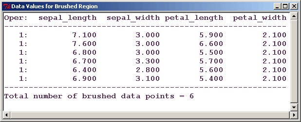
Back to top
Command - Flat Parallel Coordinates Brush Toolbox:
Function:
Raise the Flat Glyphs Brush Toolbox so that you can change the flat brushes in this toolbox in the form of parallel coordinates.
Operation:
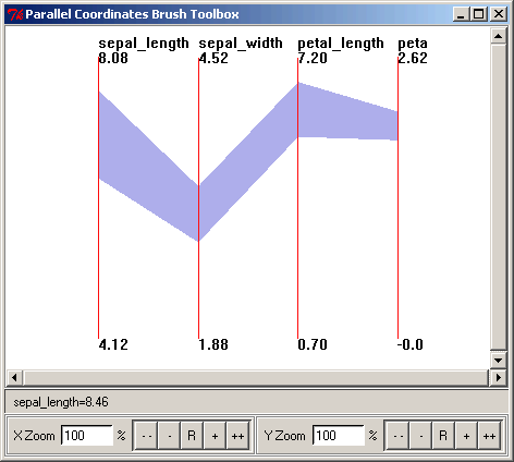
You can control the brushes in the same way as in the display of the main window. The brushes in the toolbox and other displays ???
Back to top
Command - Flat Glyphs Brush Toolbox:
Function:
Raise the Flat Glyphs Brush Toolbox. You can change the flat brushes in this toolbox in the form of glyphs by right mouse clicking or dragging and dropping.
Operation:
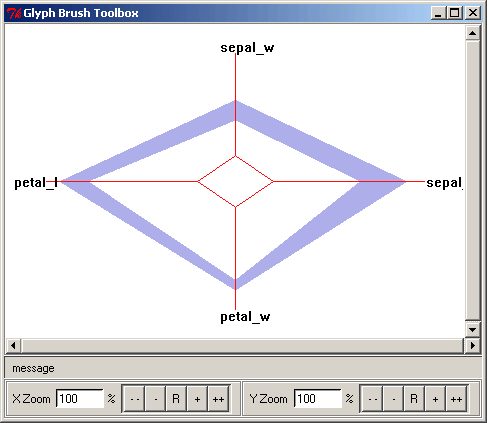
Back to top
Command - Flat Dimensional Stacking Brush Toolbox:
Function:
Raise the Flat Parallel Coordinates Brush Toolbox. You can change the flat brushes in this toolbox in the form of dimensional stacking by right mouse clicking or dragging and dropping.
Operation:
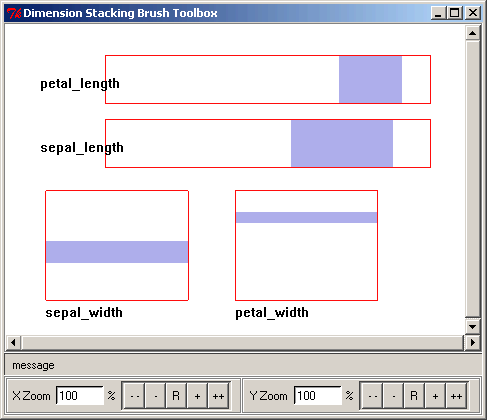
Back to top
Command - Structure-Based Brush for Hier Displays:
Function:
Raise the Structure-Based Brush Dialog. You can control the structure-based brush for the hierarchical displays in this dialog. For detailed information of the structure-based brush and hierarchical displays, please refer to Term Explanation in the help.
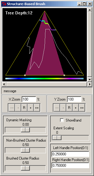
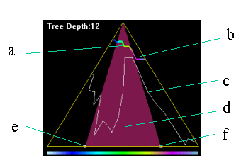
a: brushed cluster radius
b: non-brushed cluster radius
c: hierarchy contour
d: brushed region
e: left handle
f: right handle
Operation:
a. Change cluster radius
There are two ways to change the brushed cluster radius:
1. drag and drop the scaling bar under the label of "Brushed Cluster Radius" in the dialog.
2. Click on the display in the dialog. Here is an example:
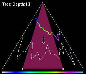
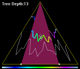
Place the cursor in the brushed region. Click the right mouse button.
There are also two methods to changed the non-brushed cluster radius:
1. drag and drop the scaling bar under the label of "Non-Brushed Cluster Radius".
2. Click on the display in the dialog. Here is an example:
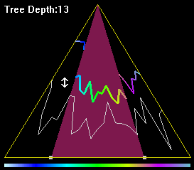
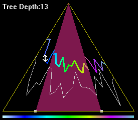
Place the cursor in the non brushed region. Click the right mouse button.
b. Change Brushed Region
You can change the brushed region by changing the left handle, changing the right handle, or changing them together.
To change the left handle, you can either input the new left handle position in the entry under the label of "Left Handle Position", or drag and drop on the display. Here is an example:
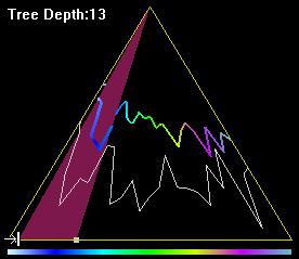
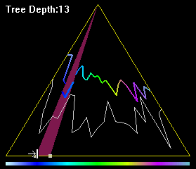
Place the cursor on the left handle. Drag and drop the cursor to a new position.
To change the right handle, you can either input the new right handle position in the entry under the label of "Right Handle Position", or drag and drop on the display. Here is an example:
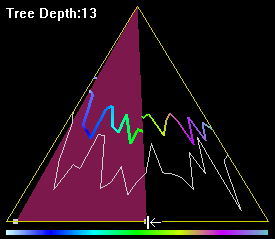

Place the cursor on the right handle. Drag and drop the cursor to a new position.
To change the left and right handle together, drag and drop the cursor in the display as the example:
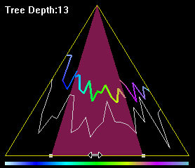
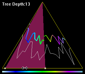
Place the cursor between the left and right handle. Drag and drop the cursor to a new position.
c. Show/hide bands
Check/uncheck the "ShowBand" check button to show or hide bands of the clusters in the hierarchical displays.
d. Extent Scaling
Drag and drop the scaling bar under the label of "Extent Scaling" change the size of the bands to reduce overlap in the hierarchical displays. When the value is 0, the bands are of the original sizes. Otherwise the bands have been decreased.
e. Dynamic Masking
Drag and drop the scaling bar under the label of "Dynamic Masking" to fake the brushed clusters or the non-brushed clusters in the hierarchical displays. When the value is 0, no clusters are faked. When it is negative, the brushed clusters are faked. When it is positive, the non-brushed clusters are faked.
Back to top
Cascade - Structure-Based Brush Semantics:
Function:
Change the semantics of the structure-based brush.
There are two semantics of the structure-based brush:
1. All - A cluster is brushed if and only if all the leaf nodes of that cluster at the brushed radius are included in the brushed region.
2. Any - A cluster is brushed as long as any leaf nodes of that cluster at the brushed radius are included in the brushed region.
Operation:
To select the All semantic, click "All" in the cascade.
To select the Any semantic, click "Any" in the cascade.
Menu: Backend
- Introduction to Prefteching Feature
- Connect Database
- Disconnect Database
- Prefetcher
- Pre-fetcher Strategy
Introduction to Prefetching Feature
Loading of data from slow persistent memory (disk storage) to main memory represents a bottleneck for current interactive visual data exploration applications, especially when applied to huge volume of data. Semantic caching of queries at the client-side can significantly improve the performance of such interactive applications. We hence propose to augment the semantic caching techniques by applying prefetching. The system predicts the user’s next requested data and loads the data into the cache as a background process before the next user request is made. However, a given pre-fetching technique is not always able to correctly predict changes in a user’s navigation pattern. Especially, as different users may have different navigation patterns, implying that the same strategy might fail for a new user. Thus for utilizing the adaptation, we introduce a concept of strategy selection to allow the choice of pre-fetching strategy to change over time both across as well as within one user session.
At present, Pre-fetching Feature only work in hierarchical view.
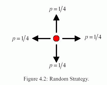
Random Strategy
As shown in Figure 4.2, strategy S1 (random) is based on randomly choosing the direction in which to prefetch next. The directions are either lateral (left or right at the same level in hierarchy) or vertical (increase or decrease level of detail). Our visualization tool only allows manipulation in one of those four directions (using six possible operations).
This strategy is appropriate when the predictor either cannot extract prefetching hints or provides hints with a low confidence measure.
Direction Strategy
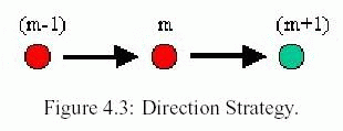
Strategy S2 (direction) is analogous to the sequential prefetching scheme. This direction strategy assumes that the most likely direction of the next operation can be determined. It is intuitive, for instance, that the user will continue to use the same navigation tool for a while before changing to other one. In our system, each navigation tool of the structure-based brush happens to precisely control one direction only. Based on a user’s past explorations, the predictor would assign probabilities to all the four directions. The prefetching strategy (S2) then is to “prefetch data in the direction” currently with the highest probability.
As depicted in Figure 4.3, if (m-1) and m are the last two directions navigated into by the user, then he direction strategy may predict (m+1) as the next direction to be visited by the user in the same direction of the previous two movements.
Focus Strategy
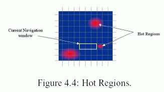
Strategy S3 (focus) uses information about the most probable next direction (by keeping track of user’s previous movement) as well as hints about regions of high interest (hot regions, as depicted in Figure 4.4) in the data space as identified based on prior navigations of this same data by other users. We found the hot regions for each user by keeping the statistics of the regions visited by the user during the past explorations, and then maintaining all the regions that have frequency of visits above a particular threshold as hot regions. This strategy will continue to prefetch data in the given direction using the above mentioned direction heuristics. However, when a hot region is around the current navigation window, the prefetcher switches from the default direction prefetching to prefetch in that now more desirable direction. The hypothesis is that the user will likely stop at such a region of interest to explore those hot regions only if she got close enough to notice it.
Command - Connect Database:
Function:
Connect to database and enable prefetching feature.

Operations:
- Input User Name
- Enter Password
- Enter the DSN Source
- click Connect button, it will connect to database. If connection is successful, prefetching feature will be enabled.
Tips:
- Configure ODBC DSN Source before connection.
- If connection fails, "Connection Exception" message will be shown in status bar.
If connection succeeds, "Connected to database successfully" message will be shown in status bar.
Command - Disconnect Database:
Function:
Disconnect to database and disable prefetching feature.
Operation:
- Select "Disconnect Database" option.
Tips:
After disconnect to database, Xmdv Tool will automatically use data from file.
Command - Prefetcher:
Function:
It is not used in this version. Prefetching Feature will be enabled after connection to database.
Command - Prefetcher Strategy:
Function:
Select one Prefetcher Strategy from the list: No Prefetcher, Random, Direction and Focus.
Operation:
- Select "Prefetcher Strategy" and click on one of the option to select that option.
Dialog: Dimension Reduction
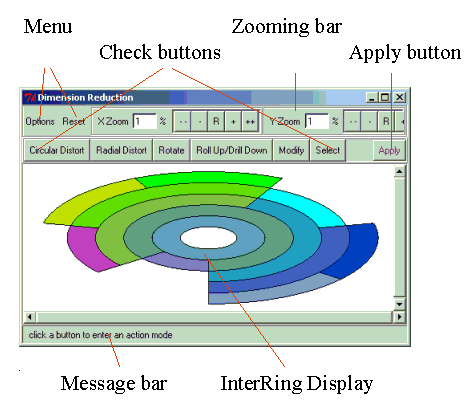
- Introduction to the Visual Hierarchical Dimension Reduction (VHDR) approach
- Menu
- Buttons
- Message bar
For more detailed information, please read our on-line documents:
InterRing: An Interactive Tool for Visually Navigating and Manipulating Hierarchical Structures
Visual Hierarchical Dimension Reduction for Exploration of High Dimensional Datasets
Introduction to the Visual Hierarchical Dimension Reduction (VHDR) approach
Visual Hierarchical Dimension Reduction (VHDR) aims to help users handle high dimensional data by generating meaningful lower dimensional spaces with user interactions. VHDR is composed of the following steps:
Step 1: Dimension Hierarchy Generation
First, all the original dimensions of a multidimensional data set are organized into a hierarchical dimension cluster tree
(the tree you see in the InterRing display) automatically according to similarities among the dimensions. Each original dimension is mapped to a leaf node in this tree. Similar dimensions are placed together and form a cluster, and similar clusters in turn compose higher-level clusters.
This step has been finished when the Dimension Reduction dialog pops
up.
Step 2: Dimension Hierarchy Navigation and Modification
Next, users can navigate through the hierarchical dimension cluster tree in order to gain a better understanding of it. Users can also interactively modify the hierarchy structure. The hierarchical dimension cluster tree is visualized
in the Dimension Reduction dialog. It is displayed using a radial space-filling
technique named
InterRing, which contains a suite of navigation and modification tools. In the
following sections of this help file, the tools will be introduced.
Step 3: Dimension Cluster Selection
Next, users interactively select interesting dimension clusters from the hierarchy in order to construct a lower dimensional subspace. Several selection mechanisms are provided in InterRing to facilitate dimension cluster
selection, which will be introduced in the later sections. Selected clusters are
highlighted using the system highlighting color.
Step 4: Representative Dimension Generation
In this step, a representative dimension (RD) is automatically created for each selected dimension cluster. The selected dimension clusters construct the lower dimensional space through these
RDs. RDs are selected to best reflect the aggregate characteristics of their associated clusters.
In this release, for a non-leaf node, the RD is the average of all the original dimensions in the
cluster. For a leaf node, the RD is the dimension itself. Users
can select one leaf node of a cluster instead of the cluster itself so that
the generated lower dimensional space could be more meaningful.
Step 5: Data Projection and Visualization
Finally, the data set is projected from the original high dimensional space to a lower dimensional space (LD space) composed of the RDs of the selected
clusters after the user clicks the "Apply" button in the dialog. We call its projection in the LD space the
mapped data set. The mapped data set is viewed as an ordinary data set in the LD space and
is visualized using the current multidimensional visualization technique in the
main window. You can also change the current visualization technique freely as
you can do for the original data set. In order to provide further dimension cluster characteristics in the LD space, such as the dissimilarity information between dimensions within a cluster, we attach the dimension cluster characteristics information to the mapped data set and provide the option to display it.
We call this dissimilarity visualization. We can perform dissimilarity visualization from two different viewpoints: from that of the individual data items, or from that of the whole data set. We name the former the ``local degree of dissimilarity (LDOD)" and the latter the ``global degree of dissimilarity (GDOD)". They are defined as follows:
LDOD - the degree of dissimilarity for a single data item in a dimension cluster. We use a mean, a maximum, and a minimum value to describe it. The mean is the mapped image of the data item on the representative dimension. The minimum and the
maximum are the minimum and maximum values among the values of the data item on all the original dimensions belonging to the dimension cluster. Note that all the dimensions have been normalized so values lie between 0 and 1.
GDOD - the degree of dissimilarity for the entire data set in a dimension cluster. It is a scalar value and can be calculated according to the similarity measures between each pair of the dimensions in the cluster. We use a simplified approach, namely, we use directly the radius of a dimension cluster as its GDOD. A dimension cluster radius is initially assigned as the similarity threshold of the iteration in which the dimension cluster is formed in the VHDR automatic dimension cluster approach.
In the Menu.Options.Dissimilarity Display section, we will introduce the dissimilarity displays in this release and introduce how to select them.
Back to top
Buttons:
There are a group of check buttons in the dialog. Each of them represents a mode of the InterRing display. With a button checked, the InterRing display enters the mode the check button represents and allows certain interactions to happen in it. You can click to check a button, and click it again to uncheck it.
Circular Distort:
In this mode, users can increase the sweep angles of the interested nodes. You can perform the distortion in two modes: the non-pin mode and the pin mode (to switch between them, use Menu->Options->Circular Distort).
In the non-pin mode, directly drag and drop the edge of the interested nodes in the InterRing display to increase or decrease them using the left mouse button.
In the pin mode, firstly click your interested nodes using right mouse button to pin them, then drag and drop their edges to increase or decrease them using the left mouse button. When you pin a node, the previous pinned node will be automatically unpinned.
Radial Distort:
In this mode, users can increase the radius of the interested levels.
Firstly, click your interested level using the right mouse button to pin it. Then drag and drop it edges to increase or decrease its radius using the left mouse button. When you pin a level, the previous pinned level will be automatically unpinned. You can also directly click or drag and drop the left mouse button without pinning any node to distort the nodes that are closest to the cursor.
Rotate:
In this mode, users can rotate the InterRing display by clicking on InterRing display. Click with left mouse button to rotate anti-clockwise. Click with right mouse button to rotate clockwise.
Roll up/Drill down:
In this mode, users can hide/show sub-branches of the tree in the InterRing display by clicking on the root node of the sub-branches. Click a node to hide the sub-branch rooted at it. Click it again to show the sub-branch expanded out.
Modify:
In this mode, users can change the tree structure. You can drag the root of a sub-branch and release it at a node that you want to be its new parent node using you left mouse button.
Select:
In this mode, users can select nodes in the tree. These nodes are the dimension clusters that will construct the new lower dimensional space after you click the Apply button.
To select a node, click it using the left mouse button. To unselect it, click it again. Or you can click the right mouse button on a node, than a "Select" dialog will pop up. Change the scaling bar in it and click OK to select multiple nodes in the sub-branch rooted at that node.
Selected clusters are highlighted using the system "highlight-1" color (system colors are the colors in the "Color Requester" dialog; you can change colors in this dialog.).
Apply Button:
If you have selected some nodes in the InterRing display, you will get you new lower dimensional space in the display of the main window. It is composed of the dimension clusters you selected in the InterRing display.
Back to top
Menu:
Options->Dissimilarity Display:
Raise the Dissimilarity Display dialog to select different methods to convey dimension cluster characteristics when visualizing the data set in lower dimensional spaces.
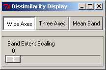
Wide Axes
You can select the "Wide Axes" button if you are in the (flat or hierarchical) Parallel Coordinates or (flat or hierarchical) Scatterplot Matrices mode.
With this button selected, if you are in the Parallel Coordinates mode, the axis width of a representative dimension is proportional to the GDOD of the dimension cluster it represents. A wider axis represents a dimension cluster with a larger GDOD. In the flat scatterplot matrices, GDOD is mapped to the width of the frames of the plots.
Three Axes
You can select the "Three Axes" button if you are in the flat Parallel Coordinates, flat Scatterplot Matrices, or flat star glyph mode to visualize LDOD.
In the flat Parallel
Coordinates mode, two extra axes are displayed around a representative dimension to indicate the minimum and maximum of the corresponding dimension cluster for every data point.
Good correlation within a cluster would manifest itself as nearly horizontal lines through the 3 axes, while lines with steep slope indicate areas of poor correlation.
In the flat Scatterplot Matrices mode, if you select the "Three Axes"
button, diagonal plots will be used to represent LDOD.
The minimum and maximum of the dimension cluster to the x and y coordinates of the diagonal plot of its representative dimension. Thus in the diagonal plots, if a point has an equal maximum and minimum, it will be represented as a point on the diagonal. On the contrary, if a point has a large LDOD, which means there is a large difference between maximum and minimum and thus a large difference between its x and y coordinates, it will lie a significant distance from the diagonal. Thus a plot along the diagonal of the matrix with points spread out in the plot away from the diagonal indicates low correlation within that dimension cluster.
In the flat Star
Glyph mode, the minimum and maximum of the dimension clusters are visualized
using the system "Grid1" and "Grid2' color. The length of the
line segment from the star center to the beginning of the "Grid1"
color is proportional to the minimum value of the cluster. The length of the
line segment from the star center to the end of the "Grid1" color is
proportional to the mean value of the cluster. The length of the line segment
from the star center to the end of the "Grid2" color is proportional
to the maximum value of the cluster.
Mean Band
You can select the "Mean Band" button if you are in the flat Parallel Coordinates mode. A band is added to each data point ranging in width from the minimum to the maximum for each representative dimension. You can reduce the overlaps using the "Band Extent Scaling" scroll bar in the Dimension Reduction dialog.
Options->Axis Color:
You can select Uniform Color or Node Color for the lower dimensional space display. If you choose Uniform Color, then all the axes in the lower dimensional space display will be the system "Grid1" color. If you choose Node Color, the axes in the lower dimensional space display will be the same colors of their corresponding nodes in the dimension hierarchy shown in the InterRing display.
Options->Circular Distortion:
To choose from the Non-Pin or Pin mode when perform the circular distortion.
Options->Visual Feedbacks:
To enable/disable circular distortion feedback, roll up/drill down feedback, and show/hide selected nodes' name.
Options->Selection Mode:
To choose from the selecting according to Entries mode or the according to Radius mode..
Options->SBBrushing Mode:
To switch the structure-based brushing mode between "cover all leaves" and "leaves only and filter out similar leaves".
In the "cover all leaves" mode, for each leaf node in the sub-branch that has been applied structure-based brushing, either itself, or one of its ascendant will be selected. While in the other mode, only leaf nodes will be selected. If there are several leaves that are similar to each other according to the dissimilarity threshold, only one of them will be selected. Unimportant leaves will also be filtered out.
Options->Reordering:
To reorder the dimension hierarchy according to their importance...
Options->Dimension Spacing:
If dimension spacing is on, after the "apply" button is pressed, the dimensions in the Paralle Coordinates and Star Glyphs displays will be placed according to the similarities between adjacent dimensions. The more similar two adjacent dimensions are, the more close they are to each other.
Reset ->Color Reset:
To reassign colors to all nodes of the dimension hierarchy according to the current tree structure. It can be used after you modify the hierarchy.
Reset->Circular Distortion Reset:
To reassign sweeping angles to all nodes of the dimension hierarchy according to the current tree structure.
Reset->Radial Distortion Reset:
To reassign radius to all levels of the dimension hierarchy according to the current tree structure.
Reset->Selection Reset:
To unselect all the currently selected nodes.
Reset->Apply Reset:
To return to the original high dimensional space.
Back to top
Message Bar:
Message bar gives you many useful "how to do" and "what's it" hints.
Mouse Events
One of the most important methods of user interaction with XmdvTool is mouse operation. Here I list the main mouse events in XmdvTool.
- Mouse Events in Main Frame
- Common Mouse Events in All Displays
- Common Mouse Events in Flat Displays
- Mouse Events in Structure-Based Brush Displays
Common Mouse Events in Main Frame:
Roll Over the Quick Buttons:
Show the functions of the quick buttons in the message bar.
Common Mouse Events in All Displays:
Right Mouse Button Drag and Drop:
Pan the display.
Common Mouse Events in Flat Displays:
Left Mouse Button Click:
Move the closest current brush edge to the current position.
Left Mouse Button Drag and Drop:
Drag and drop the closest current brush edge to the current position.
Shift Key + Left Mouse Button Click, or Drag and Drop:
Reshape the current brush to cover all the clicked data items and the data items covered in the dragged and dropped area. In Glyphs, clicking twice means non-click.
Mouse Events Structure-Based Brush Display:
Please refer the "Structure-Based Brush" section in "Brushes Menu" help file.
Term Explanation
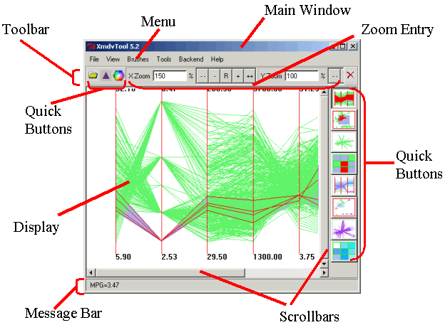
- Interface Components
- Main Window
- Menu
- Toolbar
- Zoom Entry
- Display
- Scrollbars
- Message Bar
- Quick Buttons
- Multidimensional (Multivariate) Visualization
- Flat Display Modes
- Hierarchical Display Modes
- Flat Display Brushing (flat brushing)
- Structure-Based Brushing
Interface Components
Back to top
Multidimensional (Multivariate) Visualization
Multidimensional (Multivariate) Data
Multidimensional (multivariate) data can be defined as a set of data items E, where the ith data item ei consists of a vector with N variables, ( xi1, xi2, ..., x in ). Each variable (dimension) may be independent of or interdependent with one or more of the other variable. Variables may be discrete or continuous in nature, or take on symbolic (nominal) values. Variables also have a scale associated with them, where scales are defined according to the existence or lack of an ordering relationship, a distance (interval) metric, and an absolute zero (origin).
Flat Displays and Hierarchical Displays
XmdvTool allows users to examine multidimensional data.
Four basic methods of visualizing N-D multidimensional data on a 2-D screen are provided: scatterplots, glyphs, parallel coordinates, and dimensional stacking. We refer to them as Flat Displays. A user can interactively switch between display techniques. A major tool in XmdvTool for providing insights into multidimensional spatial relations is the flat brush, which allows users to perform operations on the data points which fall within a user-specified N-D subspace of the total space defined by the data.
To explore large scale data sets, interactive hierarchical displays are provided upon the four basic displays, which are referred to as Hierarchical Displays. They are hierarchical scatterplots, glyphs, parallel coordinates, and dimensional stacking. In the hierarchical displays, all the data items in a data set is constructed into a hierarchical cluster tree. Interactive navigation tools, such as structure-based brushing, drill-down/roll-up operations, extent scaling and dynamic masking allow users to visually explore the hierarchy with user desired detail and context.
Back to top
Flat Display Techniques
Parallel Coordinates
In Parallel Coordinates, each dimension corresponds to an axis, and the N axes are organized as uniformly spaced vertical lines. A data item in N-dimensional space manifests itself as a connected set of points, one on each axis. Points lying on a common line or plane create readily perceived structures in the image. In generating the display of parallel coordinates in XmdvTool, the view area is divided into N vertical slices of equal width. At the center of each slice an axis is drawn, along with a label at the top end. Data points are generated as polylines across the N axes.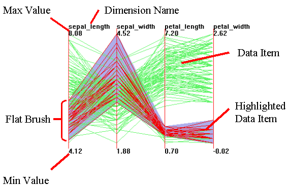
Scatterplot Matrices
Scatterplot Matrices are one of the oldest and most commonly used methods to project high-dimensional data to 2-dimensions. In this method, an grid of parallel projections of the data are generated. Each of these is a simple plot for the two dimensions it represents. The horizontal dimension of a scatterplot is controlled by the column it resides in, and likewise the vertical dimension is controlled by the row. At the top of each column and at the left of each row is a label that shows what dimensions that row / column represents.
Glyphs
The definition of a glyph covers a large number of techniques which map variables various geometric and color attributes of graphical primitives or symbols. Histograms are perhaps the most widely recognized form of glyph, where data values control the height of rectangular bars. One might even consider a scatterplot a specialized form of glyph representation, where data values control the positional attributes of a symbol. In XmdvTool, we use the star glyph pattern, which creates for each data item N rays emanating at equal angles from a point on the screen. Currently glyphs are spaced uniformly across the screen, though we might want to use 2 of the dimensions to control position. The length of each ray is determined by the data value for that dimension. A polyline is then generated to encompass the rays, forming a blob shape. The flat glyphs brush toolbox may be used as a key to the dimensions.Dimensional Stacking
Several recent techniques for multivariate display have emerged which involve projecting high-dimensional data by embedding dimensions within other dimensions. One starts by discretizing the ranges of each dimension (assigning what we term a cardinality or number of buckets for a dimension), Each dimension is then assigned an orientation (in our case, this would be horizontal or vertical) and an ordering (dimensions are said to have unique ``speeds''). The dimensions with the 2 slowest speeds are used to divide a virtual screen into sections, with the cardinalities used to determine how many sections horizontally and vertically will be generated. Each section is then used to define the virtual screen for the next 2 dimensions (slowest of the remaining dimensions), again using the cardinality to determine how to break up the virtual screen. This is repeated until all dimensions have been embedded and the data point can be mapped to its screen location. In a way, the process is similar to the manner in which the digits of an odometer move at different speeds. XmdvTool requires three types of information to project data using dimensional stacking. The first is the cardinality (number of buckets) for each dimension. The range of values for each dimension is then decomposed into that many equal sized subranges. The second type of information needed is the ordering for the dimensions, from outer-most (slowest) to inner-most (fastest). Dimensions are assumed to alternate in orientation, and the order of the dimensions in the input file is assumed to be the order for the mapping process. The last piece of information used is the minimum size for the plotted data item (the system will increase this value if the entire image can fit within the view area). Each data point then maps into a unique bucket, which in turn maps to a unique location in the resulting image. A key is provided in a separate window to help users understand the order of embedding, and grid lines of varying intensity provide assistance in interpreting transitions between buckets at different levels in the hierarchy.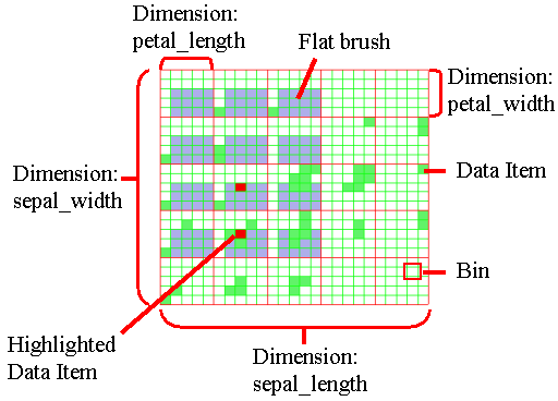
Flat Pixel Oriented Visualization:
There are two aspects that distinguish pixel oriented visualization techniques from other techniques used in XmdvTool. First, the number of data items that can be visualized without overlap is much higher than in other approaches. In general, pixel oriented techniques use each pixel of the display to represent one data value. This means that the number of data values that can be visualized at one point of time is only limited by the number of pixels on the display. A second unique feature of the technique is that the generated visualizations can be query-dependent. Query-dependency means that not only the data items fulfilling the query are visualized, but also a number of data items that approximately fulfill the query.
Back to top
Hierarchical Display Modes
Overview
Hierarchical display modes can be used to visualize large scale data sets in a multi-resolution way approach. Here is a simple description of this approach:
First, construct a hierarchical cluster tree for a data set . Similar data items are grouped into clusters, similar clusters are grouped into larger clusters. (XmdvTool automatically can automatically do this for you. So you need not worry about it. Of course, you can provide your own hierarchical tree in XmdvTool *.cg format. To learn this format, please refer to Xmdvtool website at http://davis.wpi.edu/~xmdv).
Second, visualize this hierarchy in the hierarchical display modes. To visualize a data cluster, a mean is used to indicate the average value of all the data items in the cluster, and a band is used to indicate the range of the cluster. You can visualize the data set in different level of details and highlight interesting clusters through structure-based brush. Please refer to Structure-Based Brush for Hier Displays section in Brushes Menu help file to find out how to control the bands, change levels of details and interactively play with the hierarchical displays.
If you want to learn more about the hierarchical display, please refer to Xmdvtool website at http://davis.wpi.edu/~xmdv. In the documents section we have several published papers providing detailed information on the hierarchical displays and structure-based brush.
Hierarchical Parallel Coordinates
The hierarchical parallel coordinates are derived from the flat parallel coordinates. In the hierarchical parallel coordinates, the clusters rather than individual data items are displayed. The mean of a cluster is mapped to a polyline traversing across all the axes, with a band around it depicting the extents of the cluster. The lower edge of the band intersects each axis at the minimum value of its respective cluster in that dimension. The upper edge of the band intersects each axis at the maximum value of its respective cluster in that dimension. You can imagine that if each data item included in that cluster appeared on screen, they would all be inside the band. Here is an hierarchical parallel coordinates display:
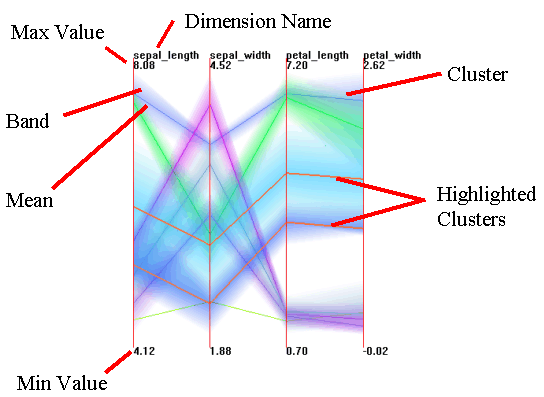
Hierarchical
Scatterplot Matrices
The hierarchical scatterplot matrices are derived from the flat scatterplot matrices. In the hierarchical scatterplot matrix, the clusters are shown in the N*N plots, where N is the original number of dimensions. The mean of a cluster is projected to the N*N plots just like how an ordinary data item in the flat form scatterplot matrix. The extent of a cluster is also projected onto the N*N plots forming rectangles around the projected mean. The projections of the same cluster on different plots are colored in the same way, which helps users link clusters from one plot to another.
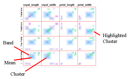
Hierarchical
Glyphs
The hierarchical
glyphs are derived from the flat glyphs . In the hierarchical glyphs, each star
glyph represents a cluster. The mean values of a cluster are mapped to the length
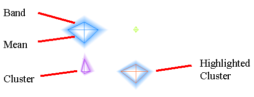
of rays emanating from a central point in the star glyph. The ends of these rays are linked to form the mean polygon. The band
around the mean polygon has two edges; one is outside the mean polygon and
another one is inside the mean polygon. The inside edge intersects each axis at
the minimum value of its respective cluster in that dimension, while the outside
edge would intersect each axis at the maximum value of its respective cluster in
that dimension if we extended the axes. Obviously, if we were to draw a star
glyph starting from this center point to present a data item included in that
cluster, this star glyph would be inside the band of that cluster.
Hierarchical
Dimensional Stacking
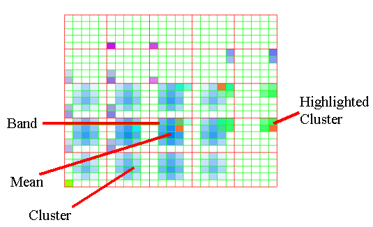
The hierarchical dimensional stacking is derived from the flat dimensional stacking. In the hierarchical dimensional stacking, the clusters replace the data items. The mean of a cluster will fall into a single small block similar to where an ordinary data item in the flat form dimensional stacking would be placed. The band of this cluster depicts the extent of the cluster. This time it is possible that some parts of the band are disjoint from others in display space due to the nature of the dimensional stacking technique.
Hierarchical Pixel Oriented Visualization :
The hierarchical visualization in XmdvTool addresses the visualization of large data sets by presenting a multi-resolution view of the data. Creation of the hierarchy preserves all the information present in the data while having access to the raw data elements. All the displays in XmdvTool have a counterpart in the hierarchical world and display the aggregate information maintained at each node in the cluster tree. The set of associated hierarchy navigation tools allows the user to discover patterns in the data set.
In order for hierarchical pixel oriented displays to show the same semantics as the flat pixel oriented displays, it is important to contrast structure-based brushing with traditional data-based brushing. In a traditional user-driven brushing operation, to specify a region of interest in a multivariate data display, the user sets upper and lower bounds for each dimension. In data-driven brushing, the user paints over groupings of interesting data. Neither of these approaches is suitable for isolating data elements which are structurally related. Rather, their focus is on the values of the data. Clearly, structure-based brushing provides new, and potentially invaluable, functionality beyond data-based brushing.
Back to top
Flat Display Brushing (flat brushing)
Flat Brush Options
Brush operations are the actions that can be performed on data selected by the brush. XmdvTool supports four types of brush operations: highlight, mask, values, and average. Each of these are explained in detail below. In order to specify a brush operation the Operation Toolbox must be used.Highlight -- This operation causes all the points covered by the brush to be displayed in a highlighting color. The highlighting color can be changed from the Color Requester dialog.
Mask -- This operation causes all points covered by the brush to be hidden from the display. This is useful when the display is cluttered and it is necessary to remove some data to view other interesting data.
Values -- This operation causes the numeric value of all points covered by the brush to be displayed in a separate popup window. This window can be opened from the main interface by selecting Data Values.
Average -- This operations causes the average value of all points currently selected by the brush to be displayed in each of the display views. In addition, if the Values operation is also selected, the numeric average is added to the end of the values in the data values window.
Brush Expression:
The brush expression is a logical expression between brushes.
Points are covered by the operation if they evaluate to TRUE for this expression.
Flat Brushing in N-D Spaces
A big problem with projecting data of a given number of dimensions to a smaller number of dimensions is that you invariably lose information regarding the spatial relationships of the data. N-D brushing (N is the number of dimensions in the dataset) is a way of recovering some of this lost information by highlighting data points which fall into a user-defined subspace. Thus, one could say ``show me the points within a (Euclidean) distance of N from a certain location.'' A brush is completely defined by its shape, size, and location. We assume a hyper-parallelepiped (a fancy name for an N-D box), and the user specifies the size of the box in each dimension. Then a location in N-D space is specified as a center point for the brush. Any data point falling within the N-D brush can have an operator applied to it, such as highlighting or masking.Each of the display methods allows the user to directly manipulate the brush. A summary of manipulation techniques for each display method follows:
Scatterplots -- The brush coverage on the scatterplot display is represented by a series of rectangular boxes, one for each scatterplot. The boxes represent the range of points that the brush covers for the two dimensions of a particular scatterplot. Each of these boxes may be manipulated using the mouse. The left mouse button can be used to resize the brush -- dragging either a corner or edge of one of the rectangular boxes will alter the brush shape. The middle mouse button may be used to recenter the brush -- dragging the box with the middle mouse button pressed will move the brush to the cursor position.
Glyphs -- The brush coverage is not displayed in the glyph view. The brush may be recentered by clicking on a glyph with the left mouse button. The brush will change location to be centered around the selected point. This is useful for finding glyphs that are similar in shape to an existing glyph.
Parallel Coordinates -- The brush coverage on the parallel coordinate display is represented by a shaded region that spans all the dimensions. The shaded region along an axis represents the range of points that the brush covers along that axis. Brush manipulation in this display works similarly to the scatterplot display. Dragging the brush with the left mouse button will resize the brush while dragging with the middle mouse button will recenter the brush.
Dimensional Stacking -- Brush coverage in this display is shown by shading all the bins that are contained by the brush. Brush manipulation in this display works similarly to the glyph display. Clicking on a point will recenter the brush to that point.
Types of Flat Brush
In XmdvTool flat brushes can have either a step edge or ramp edge. Step edge brushes allow points to either be completely inside or outside them. When a highlight operation is performed on step edge brushes, points that are completely contained by the brush are highlighted, and points not contained are painted in the normal data color.Ramped brushes do not have a discrete boundary. Instead, along each dimension there is an inner and outer brush boundary. The amount of coverage along one dimension is 1.0 inside the inner boundary and falls linearly to 0.0 at the outer boundary. When a highlight operation is performed on ramped edge brushes, points that are completely contained by the brush are drawn in the normal highlight color for that brush. Points that are partially contained by the brush are drawn in a color that is lighter as the coverage decreases. The amount of ramp of the brush is drawn as a thin line in the same color as the brush coverage on the parallel coordinate and scatterplot displays. On each of these displays, the ramp boundary may be manipulated by holding down the Control key on the keyboard and dragging with the left mouse button.
Painting
Painting is a method of creating a brush from the presented data. In order to use Painting the current brush must be both enabled and have its display attribute turned on (see Brush Toolbox). In the parallel coordinate and scatterplot displays, painting is accomplished by holding down the Shift key on the keyboard and dragging the mouse over points of interest. As long as the Shift key is held down the mouse cursor will continue to behave as a virtual paintbrush. When the Shift key is released, a brush will be generated that contains exactly all the points that were painted.Back to top
Structure-Based Brushing
This is a new variant of brushing that we have developed as a general mechanism for navigating in hierarchical space. We augment each node in the hierarchy, that is each cluster, with a monotonic value relative to its parent. This value can be, for example, the level number, the cluster size/population, or the volume of the cluster's extents. This assigned value determines the control for the level-of-detail. By choosing a continuous control variable such as the cluster size, the traversal of the tree through different levels of detail can be smooth transitions instead of abrupt screen changes.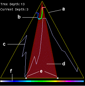
The triangular frame depicts the hierarchical tree. The leaf contour depicts the silhouette of the hierarchical tree. It delineates the approximate shape formed by chaining the leaf nodes. The colored bold contour across the middle of the tree delineates the tree cut that represents the cluster partition corresponding to a level-of-detail, for instance the cluster radius. The colors on the contour corresponds to the colors used for drawing the nodes on the main parallel coordinates display. The two movable handles on the base of the triangle, together with the apex of the triangle, form a wedge in the hierarchical space.
The brushing interaction for the user consists of localizing a subspace within the hierarchical space by positioning the two handles at the base of the triangle. The embedded wedge forms a brushed subspace within the hierarchical space. Elements within the brushed subspace may be examined at different level-of-detail.
