[Table
of Contents]
[Next]
Basic Steps of the Finite Element Method
As stated in the introduction, the finite element method is a numerical
procedure for obtaining solutions to boundary-value problems. The principle
of the method is to replace an entire continuous domain by a number of
subdomains in which the unknown function is represented by simple interpolation
functions with unknown coefficients. Thus, the original boundary-value
problem with an infinit number of degrees of freedom is converted into
a problem with a finite number of degrees of freedom, or in other words,
the solution of the whole system is approximated by a finite number of
unknown coefficients. Therefore, a finite element analysis of a boundary-value
problem should include the following basic steps:
-
Discretization or subdivision of the domain
-
Selection of the interpolation functions (to provide an approximation of
the unknown solution within an element)
-
Formulation of the system of equations ( also the major step in FEM. The
typical Ritz variational and Galerkin methods can be used.)
-
Solution of the system of equations (Once we have solved the system
of equations, we can then compute the desired parameters and display the
result in form of curves, plots, or color pictures, which are more meaningful
and interpretable.)
The first step and the last step are most relevant with the visualization
process. These 2 steps are described in greater detail below.
Domain Discretization
The discretization of the domain is the first and perhaps the most important
step in any finite element analysis because the manner in which the domain
is discretized will affect the computer storage requirements, the computation
time, and the accuracy of the numerical results. The subdomains are usually
referred to as the elements.
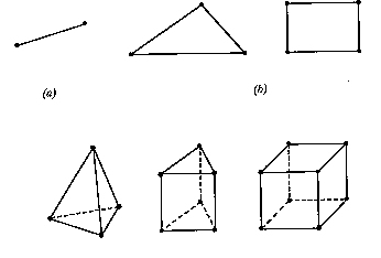
For a 1D domain which is actually a straight of curved line, the elements
are often short line segments interconnected to form the original line
[Fig2(a)]. For a 2D domain, the elements are usually small triangles and
rectangles [Fig2(b)]. The rectangular elements are, of course, best suited
for discretizing rectangular regions, while the triangular ones can be
used for irregular regions. In a 3D solution, the domain may be subdivided
into tetrahedra, triangular prisms, or rectangular bricks[Fig2(c)], among
which the tetrahedra are the simplest and best suited for arbitrary-volume
domains.
 (c)
Figure2 Basic finite elements. (a) 1D (b) 2D (c) 3D
(c)
Figure2 Basic finite elements. (a) 1D (b) 2D (c) 3D
Note that the linear line segments, triangles, and tetrahedra are the
basic one-, two-, and three-dimensional elements. Figure3 shows the finite
element discretization of a 2- and 3- dimensional domain.
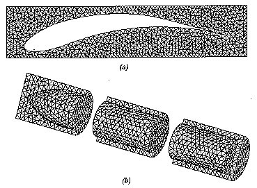 Figure 3 Examples of finite element discretization
(a) 2-D with triangular elements
(b) 3-D with tetrahedra elements
The discretization of the domain is usually considered as a preprocessing
task because it can be completely separated from the other steps. Many
well-developed finite element program packages have the capability of subdividing
an arbitrarily shaped line, surface, and volume into the corresponding
elements and also provide the optimized global numbering.
Figure 3 Examples of finite element discretization
(a) 2-D with triangular elements
(b) 3-D with tetrahedra elements
The discretization of the domain is usually considered as a preprocessing
task because it can be completely separated from the other steps. Many
well-developed finite element program packages have the capability of subdividing
an arbitrarily shaped line, surface, and volume into the corresponding
elements and also provide the optimized global numbering.
Solution of the system of equations
Once we have solved the system of equations, we can then compute the
desired parameters and display the result in form of curves, plots, or
color pictures, which are more meaningful and interpretable. This final
stage, often referred to as post-processing, can also be separated completely
from the other steps.
Index
| Next