Results

I. Problems Solved

The following tables present the problems that I have been able to solve using this program. In each case, the network, evolution strategy, training set, and test set used to solve the problem are given, as well as a brief description of the problem and comments on the success of the solution. The "Generation" field indicates how many generations the algorithm was run before producing the given solution. The first three problems were toy problems that I designed to test out the behavior of the algorithm. The remaining problems are from the Machine Learning Repository at the University of California at Irvine.
A number of these problems involve inputs and outputs that are specified, not in terms of numeric values, but as classes of attributes. For example, in the Balance Scale problem, the expected output is one of three commands: move-to-right, move-to-left, or stay-in-place. In such cases, I have arbitrarily assigned the attributes to values spread out evenly in the range 0 to 1. In the Balance Scale problem, I had move-to-left, stay-in-place, and move-to-right correspond to 0, 0.5, and 1, respectively. If a neural network were actually used to solve this sort of problem, it would be necessary to round its output to the nearest attribute. It should be clear that in the case of the Balance Scale problem, as long as the neural network's output is within .25 of the expected value, it will be producing the "correct" answer. For an output with n possible attribute values, the network must produce an answer within [1/(n-1)]/2 of the expected output in order to be correct. For two problems involving this type of output (the Image Recognition and Breast Cancer Diagnosis problems), special evaluation functions were created to determine the accuracy of the predictions made by the network. These evaluation functions are discussed in more detail in the "Comments" section of the corresponding problems.
When training neural networks to solve a problem, the choice of network architecture and activation functions is tremendously important. Unfortunately, there is no known method of choosing the best architecture for a particular problem, so the choice is largely a matter of experimentation and intuition. In the tables below, only the best networks I was able to train for each problem are presented, so that the given choices of architecture represent only one among many choices that were tried.

Problem: Sine Wave
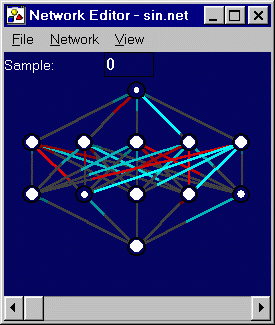
Description: The purpose of this problem was to output the sine of an angle given the angle as input.
Training Set: 25 instances
Test Set: 100 instances
Network: 1 inputs; 2 hidden layers of 5 nodes each; 1 output. Sigmoid activation functions for hidden layers; linear activation functions for inputs and outputs.
ES: (10+100)
Generation: 1502
Training Fitness: 0.024021
Test Fitness: 0.024522
Comments: Problem solved to within reasonable accuracy.
Figure 5.1: Network trained to solve the Sine Wave problem.

Problem: Squaring
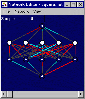
Description: The purpose of this problem was to output the square of a number between 0 and 1 given the number as input.
Training Set: 20 instances.
Test Set: 100 instances.
Network: 1 input; 2 hidden layers of 5 nodes each; 1 output. Sigmoid activation functions for hidden layers; linear activation functions for inputs and outputs.
ES: (10+100)
Generation: 501
Training Fitness: 0.004636
Test Fitness: 0.005306
Comments: Problem solved to within reasonable accuracy.
Figure 5.2: Network trained to solve the Squaring problem.

Problem: 4 Bit Parity
Description: The goal of this problem was to determine the parity (odd or even) of a four bit word, represented as four distinct boolean-valued inputs. The network is expected to produce an output of 1 for a word with odd parity, 0 otherwise.
Training Set: 16 instances (all possible combinations).
Test Set: Identical to training set.
Network: 4 inputs; 1 hidden layer of 5 nodes; 1 output. Sigmoid activation functions used for all layers.
ES: (10+100)
Generation: 3039
Training Fitness: 0.000000
Test Fitness: 0.000000
Comments: Problem solved.
Figure 5.3: Network trained to solve the 4 Bit Parity problem.

Problem: Balance Scale (Siegler76)
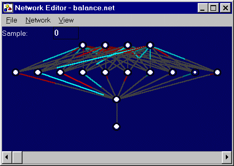
Description: This problem involved determining in which direction a pivot should be moved to balance a scale. Inputs to the problem were the two weights on the left and right side of the scale, and the distances of the two weights from the pivot. Possible outputs were move-to-left, move-to-right, and stay-in-place.
Training Set: 30 instances
Test Set: 605 instances
Network: 4 inputs; 1 hidden layer of 10 nodes; 1 hidden layer of 1 node; 1 output. Sigmoid activation functions for hidden layers; linear activation functions for inputs and outputs.
ES: (10+100)
Generation: 1000
Training Fitness: 0.008932
Test Fitness: 0.170015
Comments: Training fitness is excellent; test fitness is mediocre. Test fitness is < 1/4, so that at least 50% of the test samples will be solved correctly.
Figure 5.4: Network trained to solve the Balance Scale problem.

Problem: Balloon Classification
Description: This highly fictional problem consisted of the classification of a set of balloons according to a simple rule: a balloon is inflated if its color is yellow and its size is small. The balloon is deflated otherwise.
Training Set: 20 instances
Test Set: Identical to training set
Network: 4 inputs; 2 hidden layers of 2 nodes each; 1 output. Sigmoid activation functions for hidden layers; linear activation functions for inputs and outputs.
ES: (10+100)
Generation: 256
Training Fitness: 0.000261
Test Fitness: 0.000261
Comments: Problem solved.
Figure 5.5: Network trained to solve the Balloon Classification problem.

Problem: Predict Housing Value
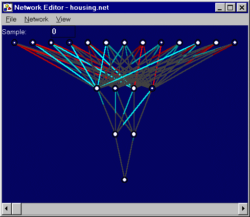
Description: The purpose of this problem was to predict the average retail value of houses in a development given 13 attributes, including average number of rooms, accessibility to highways, and property tax rates. The data were drawn from actual Boston-area housing developments (Harrison78).
Training Set: 200 instances
Test Set: 506 instances
Network: 13 inputs; 1 hidden layer of 4 nodes; 1 hidden layer of 2 nodes; 1 output. Sigmoid activation functions for hidden layers; linear activation functions for inputs and outputs.
ES: (10+100)
Generation: 6488
Training Fitness: 0.061495
Test Fitness: 0.089019
Comments: The given network well on both the training and test sets. The fitness scores corresponds to predicting the average retail price to within about $3000 and $4500, respectively.
Figure 5.6: Network trained to solve the Predict Housing Value problem.

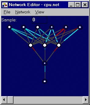
Problem: Predict CPU Performance
Description: The goal of this problem was to predict the "relative performance" of a CPU given six attributes, including cache size, MHz rating, and main memory size. The expected output is a relative performance rating, originally specified on a scale of 0 to 1000 but normalized for our purposes into the range 0 to 1.
Training Set: 60 instances
Test Set: 209 instances
Network: 6 inputs; 1 hidden layers of 3 nodes; 1 hidden layer of 1 node; 1 output. Sigmoid activation functions for hidden layers; linear activation functions for inputs and outputs.
ES: (10+100)
Generation: 244
Training Fitness: 0.019399
Test Fitness: 0.047041
Comments: Problem solved to within reasonable accuracy. The given network predicts the performance of the CPUs in the training set to within about 2%, and within under 5% in the test set.
Figure 5.7: Network trained to solve the Predict CPU Performance problem.

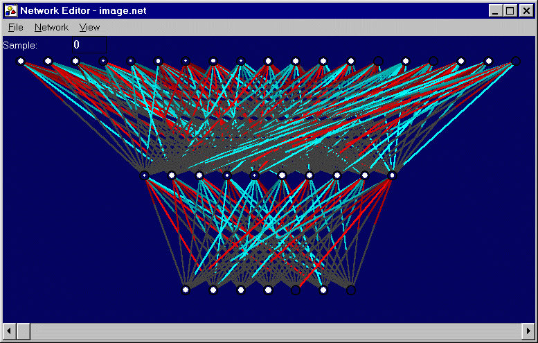
Problem: Image Recognition
Description: This problem involved the classification of images into one of seven classes: brickface, sky, foliage, cement, window, path, or grass. The image was presented to the network as a set of 19 inputs, each of which represented some aspect of the image. Inputs included the x and y coordinates of the image centroid, the mean pixel intensity, measures of contrast, and other characteristics.
Training Set: 60 instances
Test Set: 210 instances
Network: 19 inputs; 1 hidden layer of 10 nodes; 7 outputs. Sigmoid activation functions for hidden layers; linear activation functions for inputs and outputs.
ES: (10+100)
Generation: 532
Training Fitness: 90.0%
Test Fitness: 71.0%
Comments: The network performs reasonably well, though far from perfect, on both the training and test sets. A special evaluation function was created for this problem and used as the fitness score in the ES algorithm. Each of the seven outputs in this network corresponds to one of the seven image classes mentioned above. For each sample, the maximum output produced by the network is taken to be the image class into which the network predicts the sample image will fall. This is compared with the actual image class for each sample, and the fraction of correct guesses is computed as the fitness score.


Figure 5.8: Network trained to solve the Image Recognition problem.

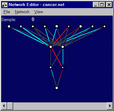
Problem: Breast Cancer Diagnosis (Wolberg90)
Description: This problem involved the diagnosis of lumps as malignant or benign based on a number of attributes, including proportion of normal nucleoli, epithelial cell size, and mitoses.
Training Set: 200 instances.
Test Set: 699 instances.
Network: 9 inputs; 2 hidden layers of 2 nodes each; 1 output. Sigmoid activation functions for hidden layers; linear activation functions for inputs and outputs.
ES: (10+100)
Generation: 299
Training Fitness: 0.099739 (96%)
Test Fitness: 0.101589 (95.6%)
Comments: The network obtains significant convergence on both the training set and the test set. The RMS error is given, as well as the result of a special evaluation function which rounds the output of the network to the nearest available category (malignant or benign), and determines the fraction of instances that the network predicts correctly. Though the results of this special evaluation are given, the networks were trained using the standard RMS fitness score. An attempt was made to train the networks using the specialized evaluation function, but this did not produce better results. The percentages given here are comparable to those obtained by Wolberg using hyperplanes (Wolberg90), and by Zhang (Zhang92) using a variety of instance-based learning algorithms.
Figure 5.9: Network trained to solve the Breast Cancer Diagnosis problem.

II. Observations

A. A Voyage into Search Space
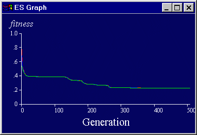

Figure 5.10: Fitness graph obtained for Tic Tac Toe problem.
The fitness graph to right was obtained by attempting to solve the Tic Tac Toe problem, which consists of nine inputs (the contents of the nine squares of a tic-tac-toe board) and one expected output, namely a 1 if the board configuration represents a win for the "X" player, and a 0 otherwise. What is interesting about this fitness graph is the multiple plateaus that exist in the search space, some lasting over 100 generations. Because of this potential, it is difficult to tell when running evolution strategies if the algorithm has reached a "stable state", from which no mutation can hope to escape, or if it simply stuck on a very large plateau. A similarly plateaud fitness graph was obtained when solving the housing value problem (described above).

B. Understanding Genetic Drift


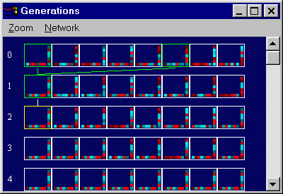
Figure 5.12: Networks trained to solve the Squaring
problem, generations 0 - 4.
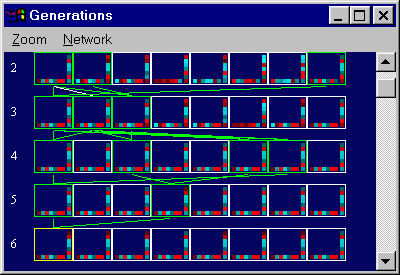
The phenomenon of genetic drift is the tendency in genetic algorithms (and in evolution strategies) for all chromosomes (in this case, encodings of the weights of neural networks) in a population to converge to roughly the same solution. Unlike in natural evolution, where multiple species compete, thrive, flourish, and die out, the populations in genetic algorithms tend to consist of a set of almost identical members, a few of which occasionally mutate into a slightly more optimal form and rapidly convert the rest of the population into their own image. To me at least, this phenomenon seems somewhat counterintuitive. I was able to more thoroughly understand it, however, by looking at the networks in a TGenerationWindow.
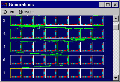
Figure 5.12 to the right was obtained using a (8+100) ES to train a population of networks to solve the Squaring problem (described above). The networks in the initial population (generation #0) have been assigned random weight values, so that initially the networks are distributed randomly throughout weight space. As shown in the figure, the 1st and 6th best networks in the initial population have combined to produce the best network in generation #1, which in turn has survived as the best network in generation #2. Already in generation #2, you will notice that the first, second, and third best networks are very similar. The reason for this is that the best network from the previous generation, even if it is only slightly better than the rest of the population, still tends to produce slightly better children that nudge out the children of other networks. In fact, as shown in Figure 5.13, the best network in each generation will be a direct descendant of the best network of the previous generation, for the first six generations of children. In generation #7 (see Figure 5.14), this pattern is broken, but by that point the networks are so similar that it doesn't matter. Subsequent generations will tend to look almost identical to generation #7, until some mutation occurs which produces a significantly better fitness score. At that point, there will be a few generations where one networks differs dramatically from the rest, but within a short time all the surviving children will be descendents of the new, mutated network.

Figure 5.13: Networks trained to solve the Squaring
problem, generations 2 - 6.
Figure 5.14: Networks trained to solve the Squaring
problem, generations 3 - 7.

C. Changing Weights & Local Optima

An interesting phenomenon occurs when using the sliding weight feature of TNVisWindow in conjunction with the backpropagation algorithm. The backpropagation algorithm, as described in the introductory chapter, conducts a gradient-based search for a local optimum in the search space. Thus, when a weight is dragged to a new location while the backpropagation algorithm is running, the network has been moved to a new location in the search space, and the local optimum toward which the algorithm was heading may no longer be the nearest one. Thus, sometimes when a weight is dragged while the algorithm is running, it will instantly "snap back" to its original location, as the algorithm returns to the same local optimum it was in before the weight was moved. But other times, dragging one weight will cause all the other weights to change in response, as the algorithm moves to a new local optimum in the search space. By adjusting various weights, it is therefore possible to determine how large a local optimum is with respect to each of the axes in weight space, providing interesting insights into the nature of the search space for a particular problem.

III. The power of NVIS

A. Topological Optimization

In first attempting to solve the 4 Bit Parity problem (described above), I made what appeared to be an impressive use of my visualization tool. Starting with a network architecture of 4 inputs, one output, and one hidden layer of 5 nodes, I observed that, after training the network to obtain a near-zero RMS error on the training set, two of the weights leading from the hidden layer into the single output were zero. This of course negated any effect that the two corresponding hidden nodes would have on the output, so it appeared that, although there were 5 nodes in the hidden layer, only 3 were actually being used. This led me to try the problem again, using only 3 nodes in the hidden layer, and I was able to obtain faster convergence than before. Looking at this new network architecture, I noticed that one of the hidden nodes was still not being used, and was able to again obtain faster convergence by reducing the number of hidden nodes to 2.
Unfortunately, these "zero" weights were actually not zero at all, and only appeared to be so due to the "black line bug" described in the "Program Implementation" chapter (see the section on TNVisWindow). The fact that removing the hidden nodes yielded faster convergence was only a matter of coincidence. After fixing this bug, I observed zero or near-zero weights going into the output layer in the course of solving several more problems. I attempted to optimize the search process by reducing the number of hidden nodes accordingly, but was able to obtain no decisive results. Thus, there is no evidence that network architecture can be optimized using this particular heuristic. Nevertheless, it may be possible using this visualization tool to perform some sort of topological optimization.

B. Designing Networks

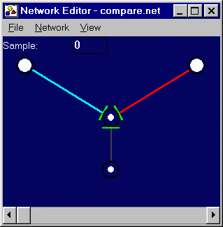
Figure 5.15: Network designed to compare its inputs.
My first attempt to solve the Balance Scale problem (described above) was not very successful. Due, as later became apparent, to the choice of network architecture and activation functions, I was unable to obtain any kind of convergence on the training set. Knowing the equation for torque from introductory physics classes, I realized that the solution to this problem consisted of two multiplications, followed by a comparison. In order to convince myself that such a problem could be solved by neural networks, I attempted to design networks that would solve the multiplication and comparison problems individually.
Figure 5.15 to the right illustrates the network I designed to solve the Comparison problem. The network multiplies its left input by a large, positive weight, and its right input by an identical weight of opposite sign. The input to the hidden node is thus a large, positive value if the left input is greater than the right input, and a large negative value otherwise. This value is passed through a sigmoid activation function to produce an output of nearly zero when the left input is less than the right, and nearly 1 otherwise. If the two inputs are equal, the network will produce an output of 0.5.
At the time I designed this network, I had not yet implemented the sliding-weight feature in TNVisWindow (described in the "Program Implementation" chapter), so that I had to edit the network file by hand. Using, this feature, however, it becomes quite easy to design a network to solve a particular problem, provided that the necessary equations are known. Moreover, it is possible to monitor the fitness score as it changes while sliding a weight, so that in designing a network, or in "tweaking" an existing network given prior knowledge about the solution to the problem, a great deal of experimentation is possible.

C. Extracting Domain Knowledge

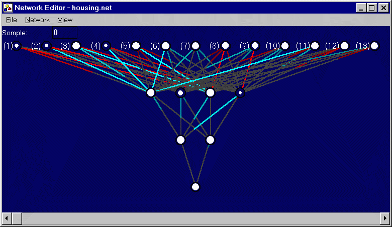
Figure 5.17 below reproduces, at a larger scale, the network depicted in Figure 5.6 above, which has been trained to solve the Predict Housing Value problem. In the case of this network in particular, a significant amount of knowledge can be gained about the factors that contribute to the retail value of a house by examining the weights that emanate from the various input nodes. For convenience, the input nodes have been numbered in the figure below (this numbering is not part of the visualization produced by TNVisWindow). The meaning of these 13 numbered inputs is defined in the following table (Figure 5.16).

 
1. Per capita crime rate (by town).
2. Proportion of residential land zoned for lots over 25,000 square feet.
3. Proportion of non-retail business acres per town.
4. Boolean variable equal to 1 if tract bounds the Charles River, 0 otherwise.
5. Nitric oxides concentration (parts per 10 million).
6. Average number of rooms per dwelling.
7. Proportion of owner-occupied units built prior to 1940.
8. Weighted distances to five Boston employment centres.
9. Index of accessibility to radial highways.
10. Full-value property-tax rate per $10,000
11. Pupil-teacher ratio by town.
12. 1000(P - 0.63)^2 where P is the proportion of blacks by town.
13. This attribute is defined in the documentation as "% lower status of the population". This either means the percentage of the U.S. population which earns less that the average person in the given housing development, or the percentage of the people in the housing development who are classified as "lower status". We will not make use of this ambiguous attribute in our analysis.
Figure 5.16: Inputs for the Predict Housing Value problem.


Figure 5.17: Network trained to solve Predict Housing Value problem, with input numbers overlaid on screen shot.


You will notice in Figure 5.17 that all the weights emanating from input node 1 (the crime rate input) are negative, suggesting that crime rates tend to reduce the value of a house. Input 6, the average number of rooms per dwelling, has all positive weights. Now being the gifted sociologists that we all are, we might already have guessed that such relationships might hold, but in principle this sort of analysis could be applied to a problem for which no prior domain knowledge exists. We can also look at the strength of the weights emanating from each input, which tells us, for example, that factors such as the proportion of homes built prior to 1940, the property tax rate, and the racial makeup of the community (inputs 7, 10, and 12, respectively) are not as important as the two zoning variables (inputs 3 and 4) or the student-teacher ratio (input 11) in determining the value of a house.
One thing that is nice about this particular network is that, with the exception of one small weight emanating from the rightmost node in the first hidden layer, all the weights in the lower two layers of this network are positive, so that the sign of the weights emanating from an input node is a direct indicator of the effect those weights have on the final output. Other networks, such as the network in Figure 5.7 trained to solve the Predict CPU Performance problem, are more difficult to analyze.