Geochemical data: heavy metals in till.  

The dataset includes 1407 samples from till (moraine) over the area of 100 x 100 kilometers. Variables are: X, Y (sample coordinates, m), Cu (copper), Co (cobalt), Ni (nickel), Pb (lead), V (vanadium), Zn (zinc) (contents, ppm=parts per million). Glacial till is a mixture of rock material, and the levels of metals in till represent the natural geochemical background. 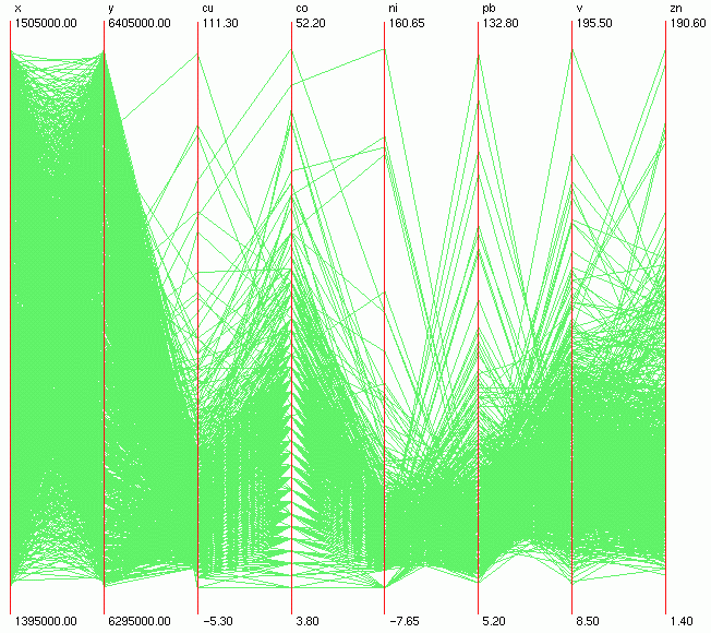There are three main rock types present within the area: granites (70% of the area), acid volcanic rocks (20%), and basic rocks (10%).The concentrations of heavy metals vary from 0 to 50-200 ppm (Figure 1). The freqency distributions of values are positively skewed, with varying number of outliers for different metals.

The first step is to identify and deal with outliers. After that, we are interested in identifying and quantifying some "multivariate fingerprints" (associations of metals) which are related to known bedrock types. Normally the geochemical data would be transformed (or outliers removed) in order to proceed with uni- and multivariate statistical analysis. The outliers may, however, contain a lot of valuable information. Analysis with GIS techniques assume interpolation of the point data, and discovering the relations between elements would mostly be based on visual displays.

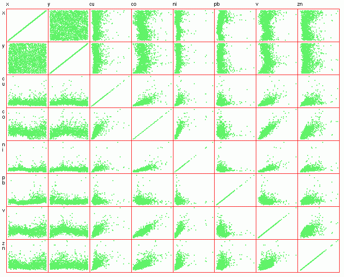
At first look, the outliers can be easily identified, and there are no visible clusters in the data (Figure 1). From the scatterplot display one can see that most elements are more or less positively correlated with each other, except for Pb (Figure 2).

Figure 1.

Figure 2.

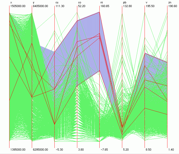
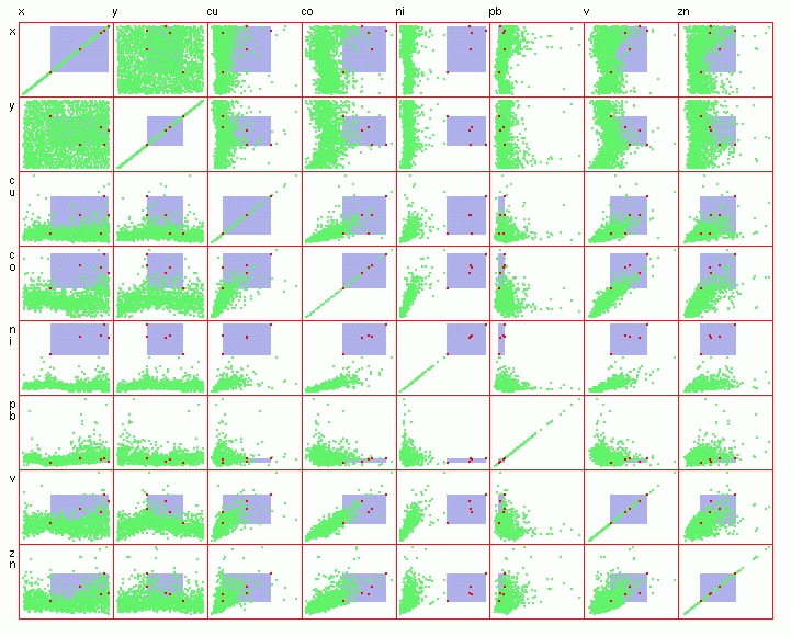
The outliers can be brushed to see if there are any atypical ones. For example, looking at the highest values for Ni, the brushed samples (Figure 3) are located mostly in the eastern part of the area (Figure 4) and certainly belong to the same type of rock, which is enriched with Ni, Co, Cu, V and Zn (basic rocks, confirmed by a bedrock map).

Figure 3.

Figure 4.

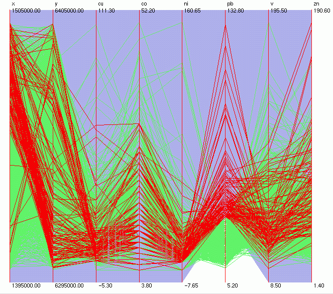
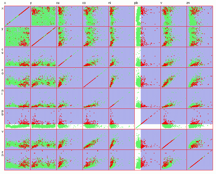
In order to study the natural geochemical anomalies within the area, we can limit the ranges of concentrations of interest to the last 10% of the samples in the high range. For example, we are interested in metal Pb and its relations with other metals (the scatterplots showed no or weak correlations). The 90th percentile value for Pb is about 35 ppm. Brushing the samples with Pb levels equal or higher than 35 ppm (Figure 5) shows that they are concentrated in the S-SE and NE of the area (Figure 6), and their "multivariate fingerprint" is a bit unclear (Figure 5). Pb and Zn seem to be correlated (that indicates some common source), but the relations with other elements are not as easy to interpret. For example, we can see that Pb and V have several kinds of relations (both positivly and negatively correlated samples), and we can try to separate those.
 

  Figure 5.

Figure 6.

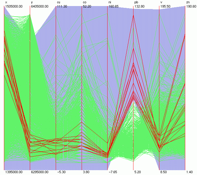
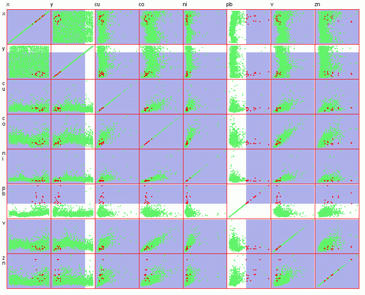
We first brush the samples that have the highest concentrations of Pb, together with low V levels (Figure 7). The scatterplot display indicates that most of those samples (Figure 8) belong to the above-mentioned S-SE cluster ( Figure 6), and contain relatively low levels of Co (less than 20 ppm).
 

Figure 7.

Figure 8.

Now, let's select all the samples with V equal to or higher than 75 ppm (the 90th percentile). The scatterplot shows a main cluster of points in the E side of the area (Figure 10). We can see that there is strong positive correlation between V and Co (Figure 9). For simplicity, we do not consider the elements Cu, Ni and Zn.
 

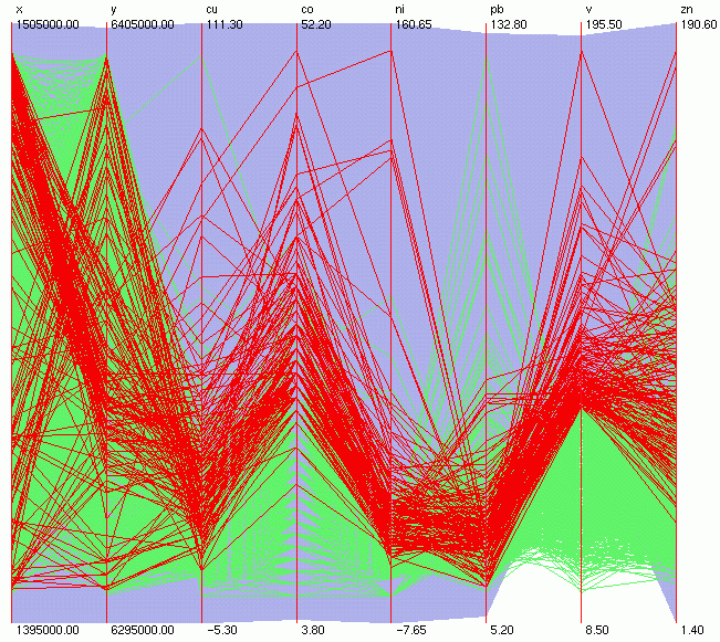
Figure 9.

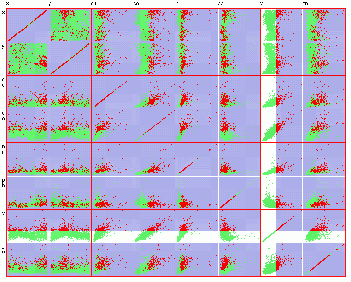
Figure 10.

From the parallel coordinates display above (Figure 9) we can notice a small cluster of samples with nearly parallel lines between the Pb and V axes. Those points have both Pb and V over their respective 90th percentile values (Figure 11, Figure 12) and belong to both the S-SE (Figure 6) and E (Figure 10) clusters. Looking closer at the first row (or first column) in the scatterplot matrix (Figure 12) we can tell that this is rather an overlap of the two anomalies than a new multivariate fingerprint, because the values of V and Co differ slightly in the two clusters.

 
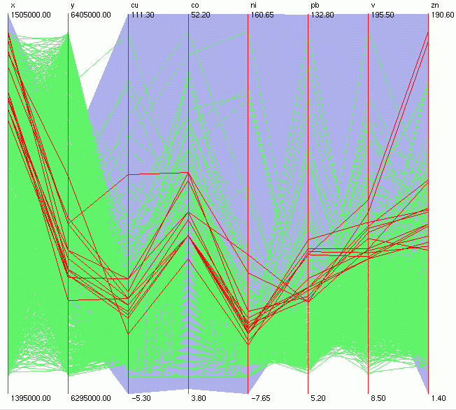
Figure 11.

 
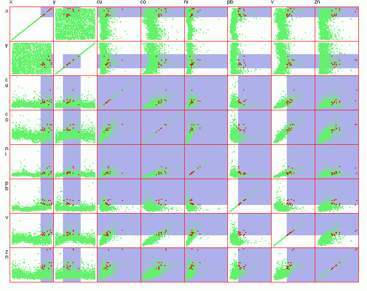
  Figure 12.

Data courtesy of SGU (the Geological Survey of Sweden).

Katrin Grunfeld

katring@geomatics.kth.se