Physical Based Techniques

Physical techniques are used by those who wish to create a more realistic cloth in both visualisation and in the actual physical characteristics of the cloth. These techniques are usually used by those trying to model certain aspects of cloth. Unlike with geometrical techniques the physical techniques are able to model the different aspects of such cloths as silk and wool. These two materials will act very differently in simular situations. These techniques are extremely useful for such people as clothing designers who are trying to model how an outfit will look like on a human model using a certain material.

C. Feynman
C. Feynamn developed a method that allowed for the modeling of draped cloth. His method represented cloth in a 3D space by using a 2D grid. His method used the equation:

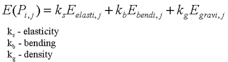
The reason behind using this function was the Feynman observed that the final shape of cloth was created when the energy of the cloth was at a minimum. The equation itself came from the theory of elastic plates.

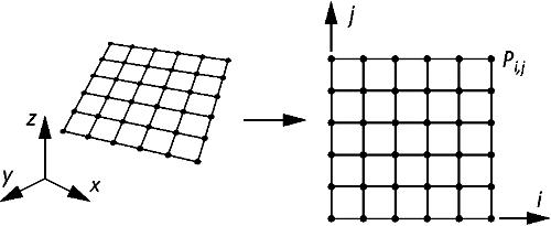
The image above show the 2D representational grid of the 3D cloth. The energy for each point P_i,j is calculated in relation to its surrounding eight points. A steepest descent method is used to find the placement of the point where the level of energy is at its lowest. Feynman used a multi-grid technique to accelerate the process of determining the state of lowest energy.

Provot
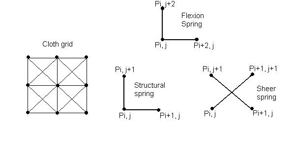
Provot used a unique method to model cloth. His method modeled cloth as springs under constrains. Because of this limitation his model did not include the draping of cloth over solid objects. The different springs that he used in his model can be seen below.

Provot's model made use of Newton's law of dynamics:

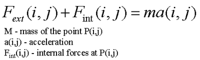
To use this model we must know what the internal forces are. Provot made use of this definition of the internal forces of the cloth.

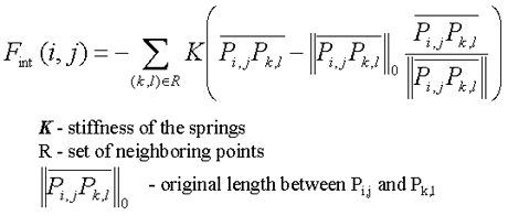
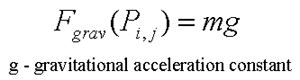
The internal forces are basically the sum of the change in point vectors multiplied by the spring stiffnesses for each neighbor of each point. The external forces for the springs were broken into three different forces. The first of which was the gravitational forces which is represented by the following equation.

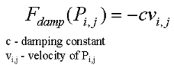
The second of these forces is the damping force represented by:

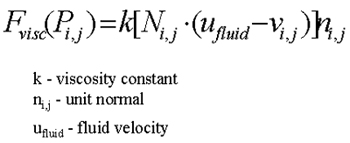
The third force that makes of the external forces is the viscosity force. This force is represented by the folowing equation.

Provot used the Euler method to integrate the first energy equation through time to be able to get the position of P_i,j at each time step. He also objserved that when a hanging cloth is simulated using the classical model, unrealistic defomations occur at the constraint points. He was able to correct this problem by detecting the deformation rate of the springs around the constraint points. If the rate became to high, the spring's elongations was limited to 10 percent.

In all Provot's model worked rather well. One benefit of the model was that using this model it was possible to model a piece of cloth flowing through any time of liquid, including water. This in itself is a great accomplishment.

A Particle Model
Many different particle models have been created in an attempt to model cloth. One of the foremost people who have worked in the area of particle modeling of cloth is David Breen. Over the years he was worked with various individuals in the developement of different particle models among other forms of cloth modeling. Particle modelling is perhaps one of the best methods for modelling cloth. The particle model that I will be discussing is more of a generic model that incorporates some of the models developed by Breen, but also used other models to help enhance various parts of the model.

The idea of this particle madel is to create fabric dependent simulations. If we want to model cloth, we want the results to be different than if we were modelling silk. Various methods have be used in attempts to recreate these characteristics. One method is to use continuum mechanics with a simulation utilizing finite elements of finite difference methods. The problem with this method is that it does not consider integral particle natures. The reason for this problem is that continuum mechanics looks at the behaviour of cloth at the macroscopic level. It assumes that only macroscopic interactions are present. In real cloth small microscopic interactions make a large impact in the overall structure and movement of cloth. We need to be ably to analyze the cloth at the microscopic level and try to make statistical assumptions about these microscopic interactions. It is rather difficult to make an exact model of these interactions. Through applying interacting-particle techniques we will attempt to catpure microscopic interactions within the material.

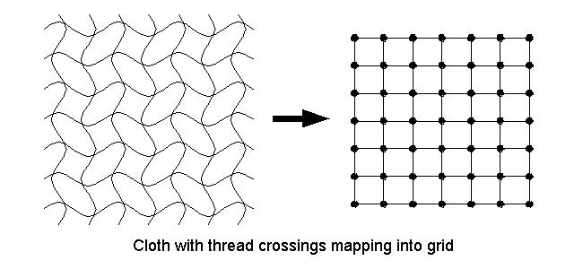
Particle Model - Capture Microstructure
Or method models the cloth as a set of particles that are located at the crossing points of the warp and weft threads. The warp threads are the verticle threads and the weft are the horizontal. The compression force amongst the weaves provide a clamp that creates an axis for the threads to bend. The image below shows the original cloth layout and the grid representation of the cloth.

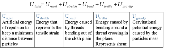
The first step in out particle model is to capture the properties of the microstructure of the cloth. The basic interactions that we want to capture are: contact, stretching, bedning and trellising. The total energy in our model is defined by the equation below. The origins of each part of the equation are given below it.

Particle Model - Repelling and Stretching
The next step is to develope equations for each part of the equation. The first part that we will look at is the repelling and stretching interactions. Normally we would use the Kawabata system to make use of the tensile strain data for all fabrics. But in the case of cloth, the tensile strain is minimal when under the stess of its own weight. This allows us to create non-cloth-specific functions for stretching and repelling. These two interactions create a steep energy well that keep the particles at a nominal distance w with their neighbors. We are able to draw the following curve and derive the following equations for the repelling and stretching energies of the particles.

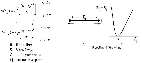
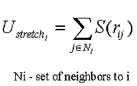
These two equations give us the repelling and stretching energies between each pair of particles. The next step is to find the total energy for a specific point i. This is simply summing over all points on the cloth. In general we do not have to sum over the whole domain of points. The reason behind this is that as the distance from i increases the function will go to 0.

An energy well is produced by the stretching potential of the neighboring points. The potential for a point i is calculated by summing the stretching potential of all neighboring points.

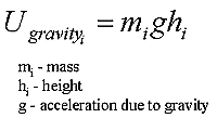
Particle Model - Gravity
The next equation that we need is the energy due to gravity. This equation is simply the mass of the point multiplied by the height and the earths acceleration constant.

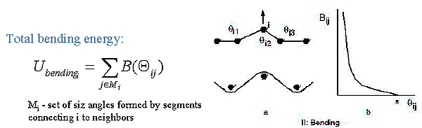
Particle Model - Bending and Trellising
We now need equations for the bending and trellising energies. Unlike the bending and stretching energies the bending and trellising properties are significant when cloth is draped. Because of this we need to base our functions on the Kawabata system. The bending of the thread is shown in the image below. It is shown along the weft direction. The warp is similar only rotated 90 degrees. The fuction for the bending energy is based on the angle between the particles in the weft and warp directions. The curve displays the bending energy against the angle between the particles.

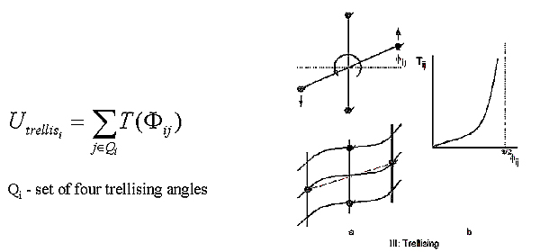
In trellising two segments are formed by joining the nearest horizontal and vertical neighbors. When the cloth drapes, then equilibrium angle of 90 degrees between neighboring particles turns into an S shape. The trellising angle is the angle that is formed between the original equilibrium line and the line segment between the current configurations of the points. The total trellising energy is calculated by adding up the total energy of the four point. These points can be seen in image a below.

Particle Model - Minimizing the Energy
Now that we can calculate the amount of energy that each particle has me must now find the state in which the particles have the lowest energy. This is done on the assumption that the the cloth will always come to rest in a state of low energy. To do this we must first write the energy equation in the terms of coordinates (U = f(x,y,z)). Both U_repel and U_stretch are functions of r_ij, where r_ij is the distance between the points i and j. r_ij is expressed as:

We then need to put the angles into terms of coordinates for use in the bending equations. This can be easily writtten as a cross product of vectors. When we do this we get that the angle theta is equal to the inverse cosine of the cross product of two vectors.

We use the same methods to come up with equations for the other angles for the bennding and trellising equations. Since we now have the energy in terms of coordinates we want to look for the following conditions:

If we differentiate the energy equations with respect to x, y and z we get simultaneous equations involving the grid elements. If we have a 50*50 grid, we will get a 50*50 simultaneious equations. These eqations will give us the location of all particles.

Particle Model - Cloth Specific Tuning
Up until this point we have created a very general model that doesn't have any specific attributes of any one type of cloth. The next step is to add different attributes to the model so that heavy wool will react differently than silk in our model. To do this we need to develop equations based on the Kawabata Evaluation System (KES). This system measures the physical and mechanical properties of cloth. To truly understand the KES one must have a fair amount of knowledge of structural mechanics. As such, I will not be going into all that much detail.

Or basic aim to com develop function B and T that give the bendng and trellising energies. The KES measures how much force is required to perform 3 types of deformations on a fabric sample. It produces plots of the forces as a function of various geometric parameters, such as the one below.

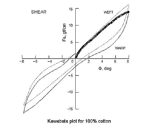
Our aim is to represent this curve using polynomials so that we can extract valus from them. To do this we need to define our trellising and bending energies.

Particle Model - Bending Energy Equations
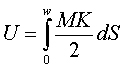
If we assume that the theory of elastic bending beams is applicable, then the straining energy dU due to the bending stored in as segment dS can be represented by.

Each particle is separated by its neighbors by the distance w. Each of these particles can be said to represent a piece of cloth. These pieces of cloth can be considered to to be beams running in parallel to one another. This assumption allows us to calculate the energy of on beam with the following equation.

If we assume that over the length of the w X w patch of cloth the bending moment and the curvature are a constent then we can use the following equation for the energy.

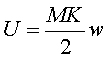
M is given in moment per unit length. Therefore the energy for the threads in the cloth can be described as.

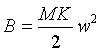
M is in terms of K derived from the Kawabat plot. This means that we still need to calculate the curvature (K). The curvature at a specific point can be considered to be a constant between 2 neighbors. We can just fit a circle betwee the 2 neighbors of a point. We then get the following equatin for K.

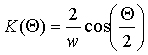
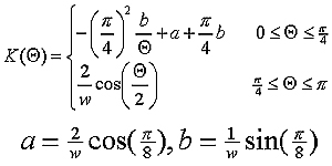
As the angle goes toward 0, K becomes 2/w. This is not physically correct. As the angle goes to 0 the thread bends back on itself creating a curvature of infinity. This is obviously not realistic. To correct this problem we assume that the equation only holds for angles between 45 and 180 degrees. For other angles we must use the following equation.

Particle Model - Trellising Energy Equations
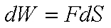
The work dW produced by a force F acting over a displacement dS is

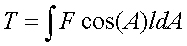
If we assume the width l is constant during shearing, the path traveled by the particle can then be defined by S = lA. Where A is the shearing angle. Therefore dS = ldA. If the force is on a circular arc, its direction is not parallel to the force. In this case, Fcos(A) is the component of force along the displacment. Thus allowing use to derive the following equation for the total energy for shearing.

For any material we can use the Kawabata curves for shearing force as a function of A and then integrate to get T.

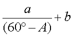
At a maximum shear of 60 degrees the shear force goes to infinity. In this case we have to use the following curve to the slope and position of the enpoint of our Kawabata curve.

Using all of the equations and techniques in this section you should be able to have a general idea of how to use a particle model to model cloth.