Fluid Simulation
Paper Generation
Main Loop
Moving Water Through the Shallow Water Layer
Updating the Water Velocities
Relaxation
Edge Darkening
Moving Pigments
Backruns
Drybrush Effects
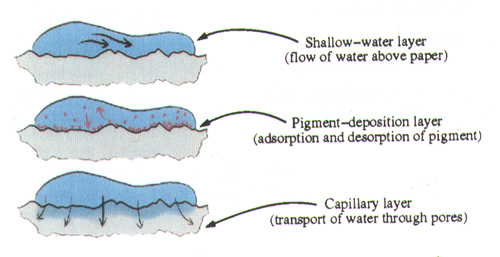
Each wash in our simulation is broken down into three layers. The first layer
is the shallow-water layer. This layer describes where the water and pigment flow
above the surface of the paper. The second layer is the pigment-deposition
layer. This layer describes the location where pigment is diposited onto and lifted up
from the paper. The final layer is the capillary layer. This layer describes the location
where water is absorbed and diffused through the paper through capillary action.
The following are the values that are used in the fluid simulations calculations.
In the simulation of the shallow-water layer the water flows acrowss the surface in a way that
is bounded by the wet-area mask. As the water flows over the paper, pigment is both lifted
from and deposited onto the paper. Each pigment k is transfered during this process. The pigment
in the shallow-water layer is denoted g^k and the deposited pigment is denoted as d^k. The
ability of the pigment to be absorbed and desorbed by the paper is effected by its density (rho),
staining power (omega) and its granulairty (gamma). The capillary layer allows for the expansion
of the wet-area mask due to the capillary flow of the water through the pores of the paper. All of
these properties are discretized over a two-dimensionl grid to be used in the final fluid
simulation.
Paper Generation
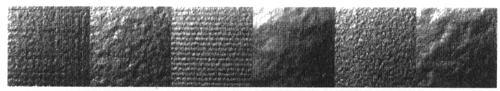
Before we can perform the fluid simulation we must be able to recreate a useful paper model. To do this
we modeled the paper as a height field and a fluid capacity field. The height field h is generated
using a selection of pseudo-random processes. The value is then scaled to be between 0 and 1. The slope of
the height field is used to modify the fluid velocity in the fluid simulations. The overall fluid
capacity c of the paper is computed from the height field using the following equation: c = h * (c_max - c_min) + c_min.
Some examples of papers textures that we created using this method can be seen below.
Main Loop

The Main Loop of our fluid simulation takes in the initial wet-area mask (M), the initial
velocities of the water in the x and y directions (u,v), the initial water pressure (p), the
initial pigment concentrations (g^k, d^k), and the initial water saturation of the paper (s).
The Main Loop loops a specific number of times. On each loop it moves the water and pigment in
the shallow-water layer, transfers pigment between the shallow-water layer and the
pigment-deposition layer, and simulates the capillary flow of the water through the paper.
Moving Water Through the Shallow-Water LayerJ
In simulating the flow of water in in the shallow water layer we must take into account certain
restraints that will allow us to create a realistic flow of the water. The flow of of the water
must follow:
- the flow must be constrained so that water remains withing the wet-area mask
- a surplus of water in one area should cause flow outward from that area into nearby regions
- the flow must be damped to minimize oscillating waves
- the flow must be perturbed by the texture of the paper to cause streaks parallel to flow direction
- local changes, such as adding water, should have global effects
- there should be outward flow of the fluid towards the edges to produce the edge-darkening effect
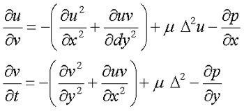
To satisfy the first two conditions we must use the folowing two equations with appropriate boudary conditions.
We implemented these equations using the UpdateVelocities subroutine that will be discussed later.
The third and fourth conditions are satisfied by adding both viscous drag (kappa) and the paper slope
(inverse delta h) to the fluid flow simulation in the UpdateVelocities routine. The final two conditions are
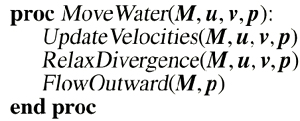
met by the use of the RelaxDivergence and FlowOutward routines. These three routines are combined together
to create the MoveWater routing which simulates the movement of water in the shallow-water layer.
Updating the Water Velocities
In order to update the water velocities we discretized the two equations discussed above on a staggered grid.
The staggered grid representation stores velocity values at the grid cell boundaries and all other values at
the grid cell centers. We used the standard notation for staggered grids in which we refer to quantities on
cell boundaries as having "fractional" indices. For example a velocity u at the boundary between
cell (i,j) and cell (i+1,j) is called u_i+.5,j. Using this notation we can denote quantities that aren't
specifically represented by averaging the values of their neighbors (p_i+.5,j = (p_i,j + p_i+1,j)/2).
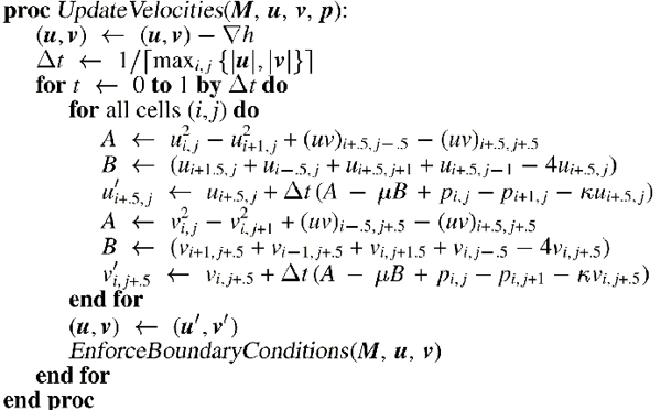
The pseudocode above represents our UpdateVelocities routine. The delta t step at the start of the routine is to ensure
that the velocities do not exceed on pixel per time step. It does this by taking the ceiling of the highest x and y
velocites of the grids. The routine then goes through every cell in our grid system an calculates a new value for u and
v, the representations of the velocities in the x and y directions. These calculations are based on the velocities of the
water in the current grid and the surrounding grids, and the viscosity (mu) and viscous drag (kappa) of the water. The
EnforceBoundaryConditions procedure sets the velocity of any pixel that is not in the wet-area mask to zero.
Relaxation
The purpose of the RelaxDivergence process is to relax the divergence of the velocity field at each time step until
it becomes less than some set tolerance Tau. It does this by redistributing the fluid into the cell's neighbors.
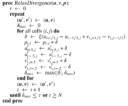
As you can see from the above pseudocode the first step is to set delta_max to 0. For each cell that the iteration
runs though delta is set to a certain percentage (Xi) of the total difference in the x and y velocities between itself and
its neighboring cell. This difference is then added to the water pressure of the cell and to the +x direction of the cell and
subtracted from the -x direction of the cell. Delta_max is then set to the maximum between itself and the delta calculated above.
If this maximum is less than the set tolerance level or the number of iterations is greater than some set N, then the function exits,
otherwise the whole process is repeated.
Edge Darkening
Edge darkening is caused by the tendency of pigments to migrate from the interior of a paint stroke towards the edges over time.
This tendency is caused cecause liquid evaporating near the boundary must be replenished by liquid from the interior. As the
liquid flows outward to fill in for the evaporating liquid, pigment is carried along with the flow of water only to be deposited by
the water near the edges of the stroke. The FlowOutward routine removes ate each time step an amount of water from each cell. More
water is removed from cells closer to the boundaries of the cells. The distance to the boundary is approximated by applying a
Gaussian blur with a K X K kernel on the wet-area mask M. The total amount of water to be removed at each time step is
based on the resulting image of the blur by the following formula: p <- p - n * (1 - M') * M.
Moving Pigments
The flow of water in the shallow-water layer effects the movement of the pigment contained within the water.
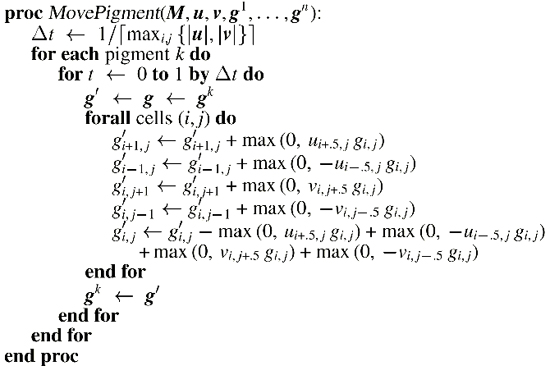
Therefore in our MovePigment routine we transfer pigment from one cell to another based on the
rate of fluid movement out of the cell. Once again you can see that delta t is calculated to limit the
velocity to one pixel per time step. The routing goes through each of the cells and checks to see if
there is a positive velocity going into that cell. If there is a positive velocity, then the velocity
multiplied by the pigment concentration in the cells neighbor is added to the cells current concentratino and
subtracted from its neighbors. By using this technique on all of the cells neighbors the routine transfers
pigment between the different cells.
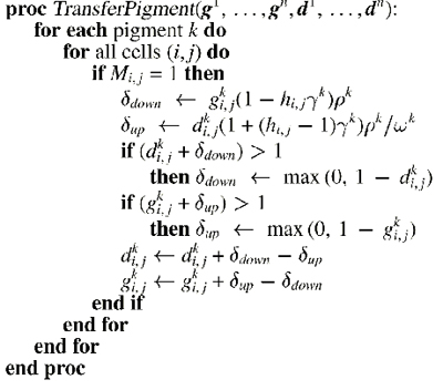
During each step of the simulation pigment is being absorbed and desorbed by the pigment-deposition layer
at a certain rate. This rate is affected by the density (rho^k) and staining power (xi^k) of the pigment.
The granulation gamma^k determines how much the paper height affects the rate of absortion and desorption.
The routing goes though each cell and checks to see if it is "wet." It then calculates how much pigment is
being absorbed by taking into account the current concentration, the grannulation and the density of the pigment.
It calculates the amount of pigment being desorbed by taking into account the grannulation, the density and the
staining power of the pigment. The routine then makes sure that the total amount of pigment either absorbed or
desorbed is less than 1. If not than the amount being absorbed or desorbed is adjusted. The final value for
the concentrations of pigment are then calculated.
Backruns
Backruns occur when a puddle of water spreads into an area that is drying but is still damp.
In this situation the movement of the water is primarily based on capillary flow instead of
inertia. In our simulation the water is absorbed from the shallow-water layer at a rate (alpha).
This water is then transfered from one cell to all of its neighbors until the cells are
saturated to capacity (c). In the SimulateCappilaryFlow routine epsilon represents the minimum
saturation that a cell must have to pass water to other cells and delta is a saturation level
below which a pixel will not receive diffusion. The first step in this routine is to add the maximum
amount of water to the cell, either the absorption rate or the most water that can fit into the cell at
the time. The next step is to go through each neighbor of each cell and transfer the water from the cell
to its neighbors if the cell has enough water to diffuse.
Drybrush Effects
The drybrush effect only occurs when the brush is applied at the proper angle and is
dry enough to wet only the highest points on the paper surface. We were able to model this
by excluding from the wet-area mask andy pixel whose height is less than a certain threshold.